Lecture 17 Factor Analysis Syllabus Lecture 01 Lecture
Lecture 17 Factor Analysis
Syllabus Lecture 01 Lecture 02 Lecture 03 Lecture 04 Lecture 05 Lecture 06 Lecture 07 Lecture 08 Lecture 09 Lecture 10 Lecture 11 Lecture 12 Lecture 13 Lecture 14 Lecture 15 Lecture 16 Lecture 17 Lecture 18 Lecture 19 Lecture 20 Lecture 21 Lecture 22 Lecture 23 Lecture 24 Describing Inverse Problems Probability and Measurement Error, Part 1 Probability and Measurement Error, Part 2 The L 2 Norm and Simple Least Squares A Priori Information and Weighted Least Squared Resolution and Generalized Inverses Backus-Gilbert Inverse and the Trade Off of Resolution and Variance The Principle of Maximum Likelihood Inexact Theories Nonuniqueness and Localized Averages Vector Spaces and Singular Value Decomposition Equality and Inequality Constraints L 1 , L∞ Norm Problems and Linear Programming Nonlinear Problems: Grid and Monte Carlo Searches Nonlinear Problems: Newton’s Method Nonlinear Problems: Simulated Annealing and Bootstrap Confidence Intervals Factor Analysis Varimax Factors, Empircal Orthogonal Functions Backus-Gilbert Theory for Continuous Problems; Radon’s Problem Linear Operators and Their Adjoints Fréchet Derivatives Exemplary Inverse Problems, incl. Filter Design Exemplary Inverse Problems, incl. Earthquake Location Exemplary Inverse Problems, incl. Vibrational Problems
Purpose of the Lecture Introduce Factor Analysis Work through an example
Part 1 Factor Analysis
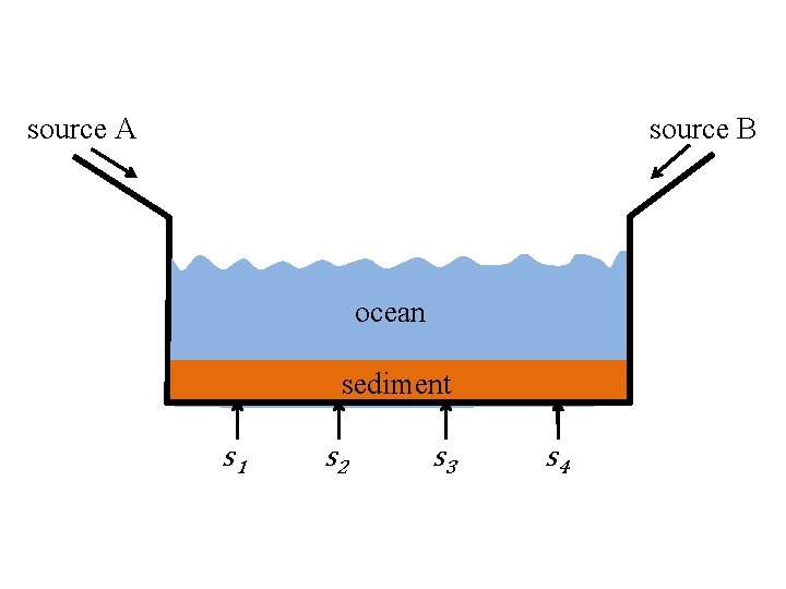
source A source B ocean sediment s 1 s 2 s 3 s 4
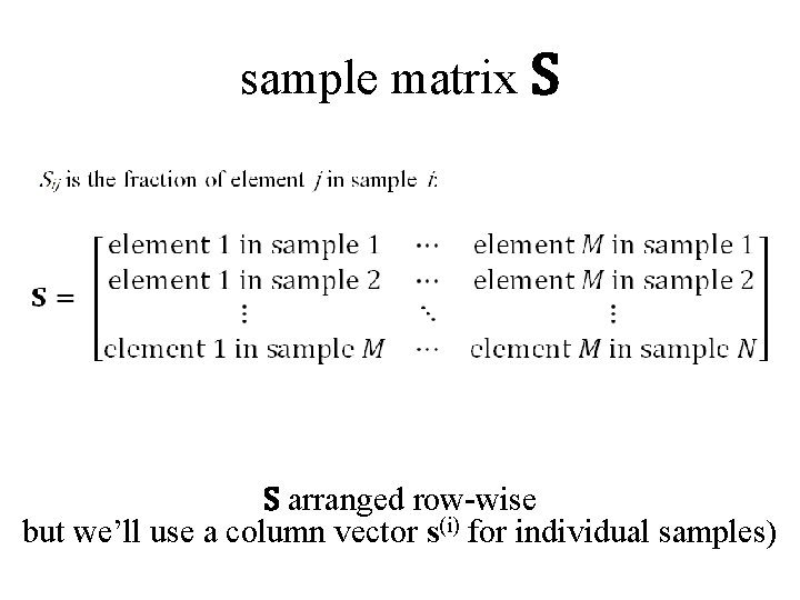
sample matrix S S arranged row-wise but we’ll use a column vector s(i) for individual samples)
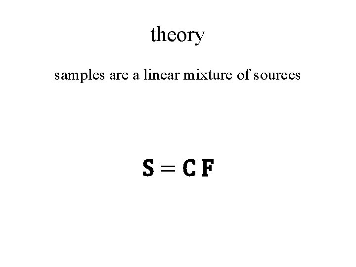
theory samples are a linear mixture of sources S=CF
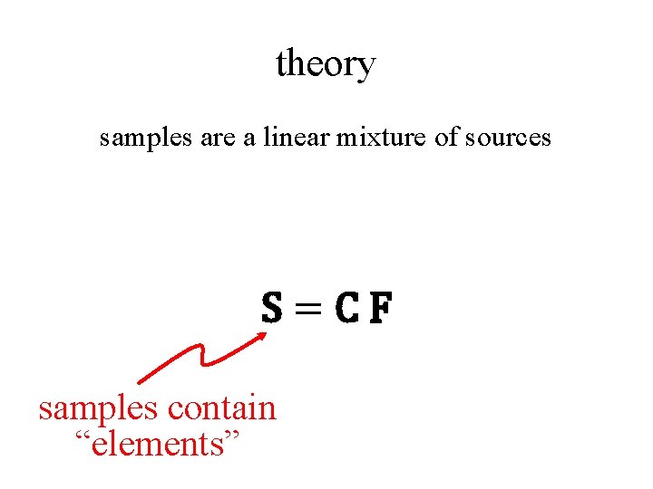
theory samples are a linear mixture of sources S=CF samples contain “elements”
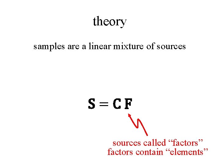
theory samples are a linear mixture of sources S=CF sources called “factors” factors contain “elements”
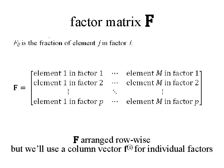
factor matrix F F arranged row-wise but we’ll use a column vector f(i) for individual factors
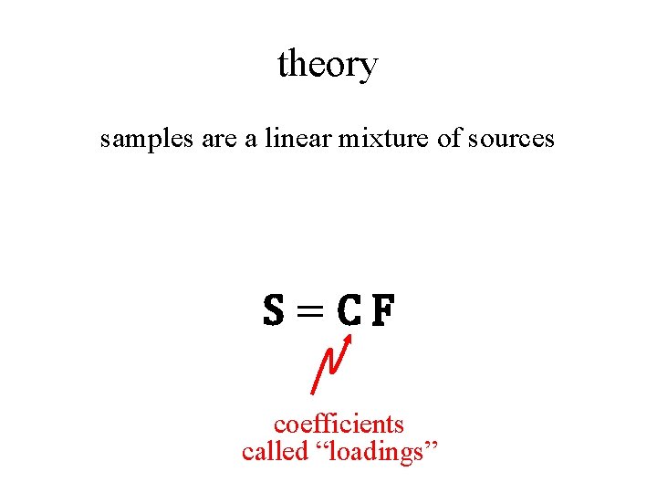
theory samples are a linear mixture of sources S=CF coefficients called “loadings”
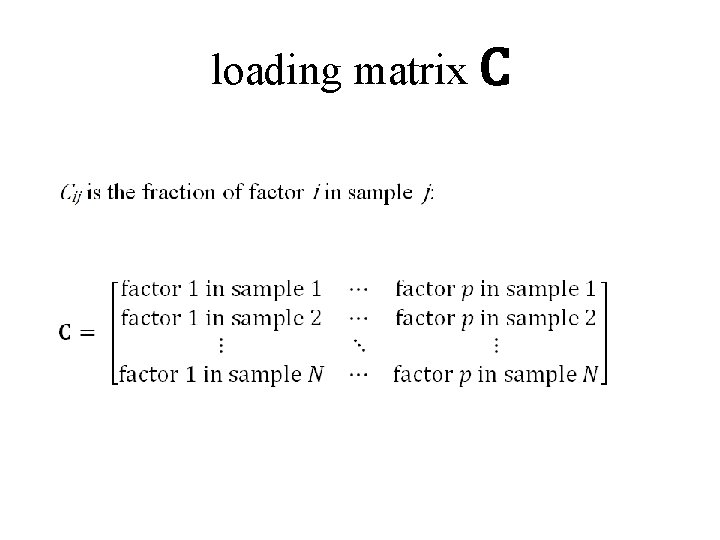
loading matrix C
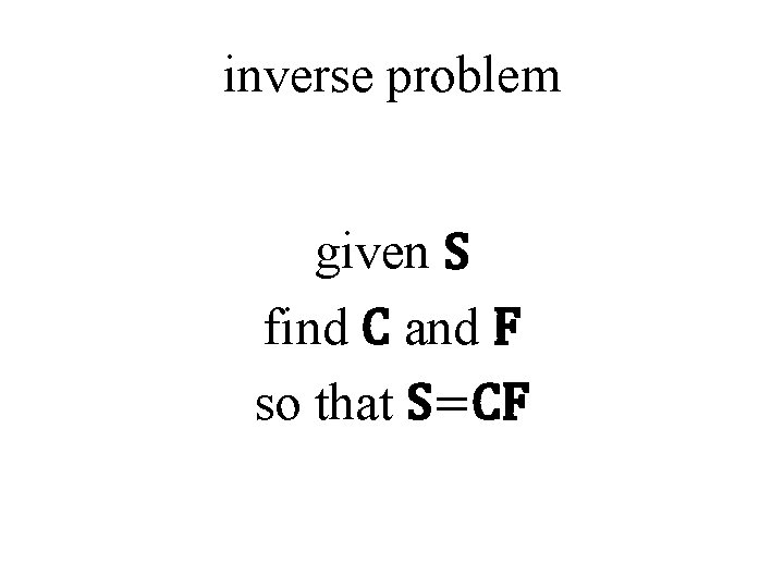
inverse problem given S find C and F so that S=CF
![very non-unique given T with inverse T-1 if S=CF -1 then S=[C T ][TF] very non-unique given T with inverse T-1 if S=CF -1 then S=[C T ][TF]](http://slidetodoc.com/presentation_image_h/9b59c64af8794bfbe7cbd06963b95474/image-14.jpg)
very non-unique given T with inverse T-1 if S=CF -1 then S=[C T ][TF] =C’F’

very non-unique so a priori information needed to select a solution
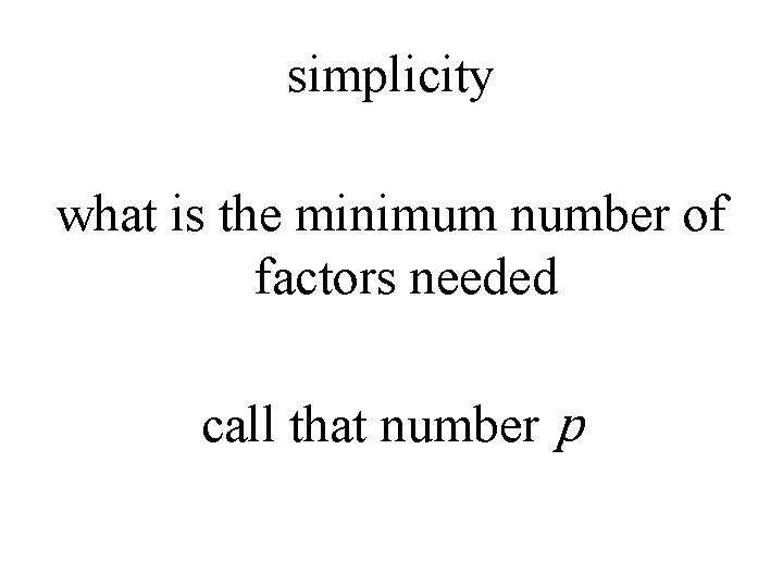
simplicity what is the minimum number of factors needed call that number p
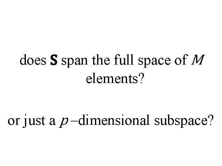
does S span the full space of M elements? or just a p –dimensional subspace?
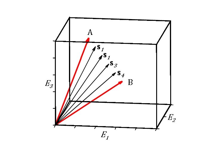
A s 1 s 3 s 4 B E 3 E 2 E 1
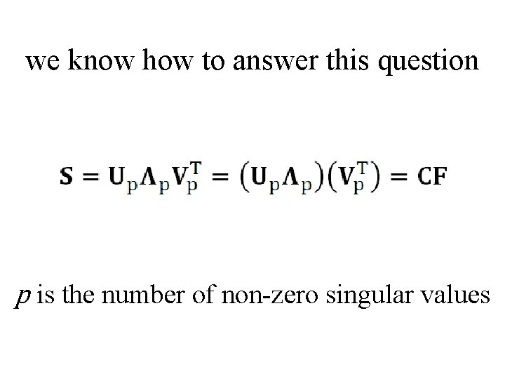
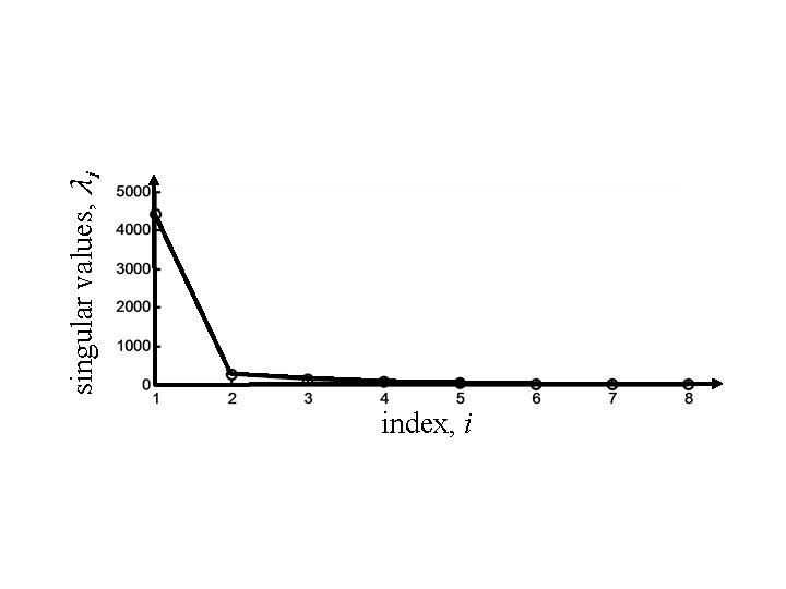
we know how to answer this question p is the number of non-zero singular values
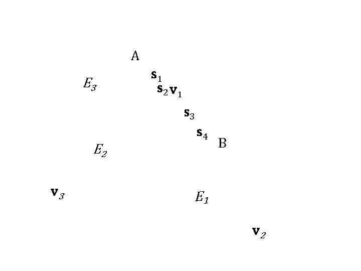
A E 3 s 1 s 2 v 1 s 3 s 4 E 2 v 3 B E 1 v 2
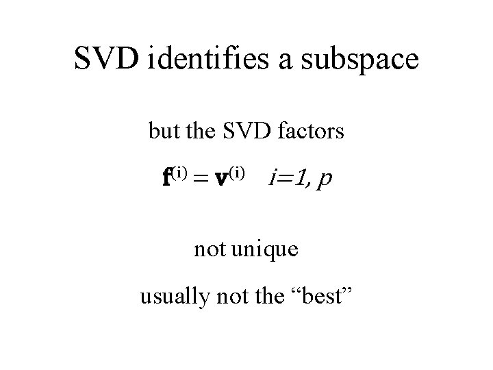
SVD identifies a subspace but the SVD factors f(i) = v(i) i=1, p not unique usually not the “best”
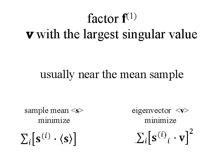
(1) f factor v with the largest singular value usually near the mean sample mean <s> minimize eigenvector <v> minimize
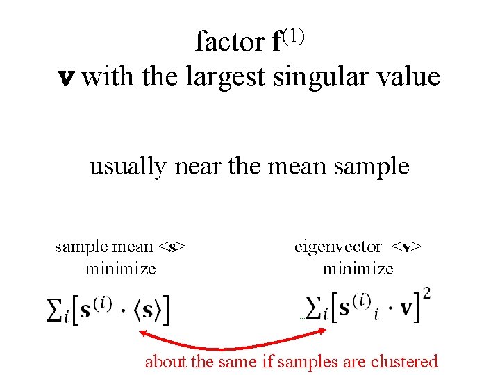
(1) f factor v with the largest singular value usually near the mean sample mean <s> minimize eigenvector <v> minimize about the same if samples are clustered
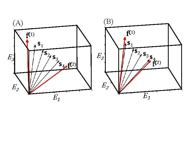
(B) (A) f(1) s 1 E 3 s 2 s 3 s 4 f(2) E 3 f(1) s 1 s 2 s 3 s 4 f(2) E 2 E 1
![in Mat. Lab [U, LAMBDA, V] = svd(S, 0); lambda = diag(LAMBDA); F = in Mat. Lab [U, LAMBDA, V] = svd(S, 0); lambda = diag(LAMBDA); F =](http://slidetodoc.com/presentation_image_h/9b59c64af8794bfbe7cbd06963b95474/image-25.jpg)
in Mat. Lab [U, LAMBDA, V] = svd(S, 0); lambda = diag(LAMBDA); F = V'; C = U*LAMBDA;
![in Mat. Lab “economy” calculation LAMBDA is M⨉M [U, LAMBDA, V] = svd(S, 0); in Mat. Lab “economy” calculation LAMBDA is M⨉M [U, LAMBDA, V] = svd(S, 0);](http://slidetodoc.com/presentation_image_h/9b59c64af8794bfbe7cbd06963b95474/image-26.jpg)
in Mat. Lab “economy” calculation LAMBDA is M⨉M [U, LAMBDA, V] = svd(S, 0); lambda = diag(LAMBDA); F = V'; C = U*LAMBDA;
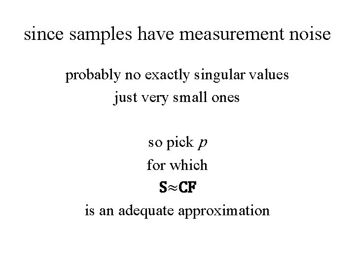
since samples have measurement noise probably no exactly singular values just very small ones so pick p for which S≈CF is an adequate approximation
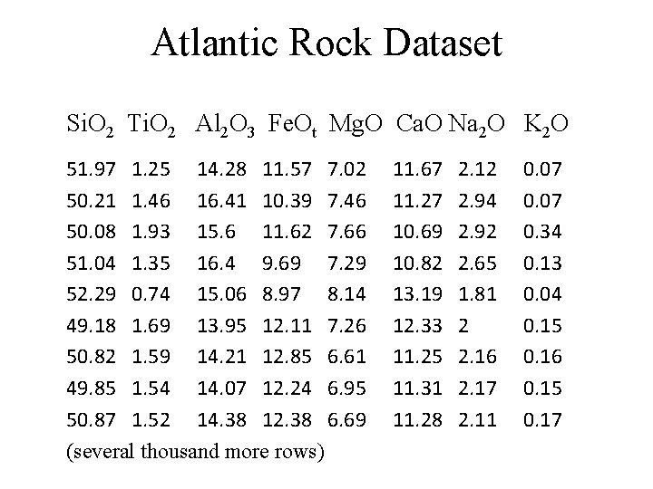
Atlantic Rock Dataset Si. O 2 Ti. O 2 Al 2 O 3 Fe. Ot Mg. O Ca. O Na 2 O K 2 O 51. 97 1. 25 14. 28 11. 57 7. 02 50. 21 1. 46 16. 41 10. 39 7. 46 50. 08 1. 93 15. 6 11. 62 7. 66 51. 04 1. 35 16. 4 9. 69 7. 29 52. 29 0. 74 15. 06 8. 97 8. 14 49. 18 1. 69 13. 95 12. 11 7. 26 50. 82 1. 59 14. 21 12. 85 6. 61 49. 85 1. 54 14. 07 12. 24 6. 95 50. 87 1. 52 14. 38 12. 38 6. 69 (several thousand more rows) 11. 67 11. 27 10. 69 10. 82 13. 19 12. 33 11. 25 11. 31 11. 28 2. 12 2. 94 2. 92 2. 65 1. 81 2 2. 16 2. 17 2. 11 0. 07 0. 34 0. 13 0. 04 0. 15 0. 16 0. 15 0. 17
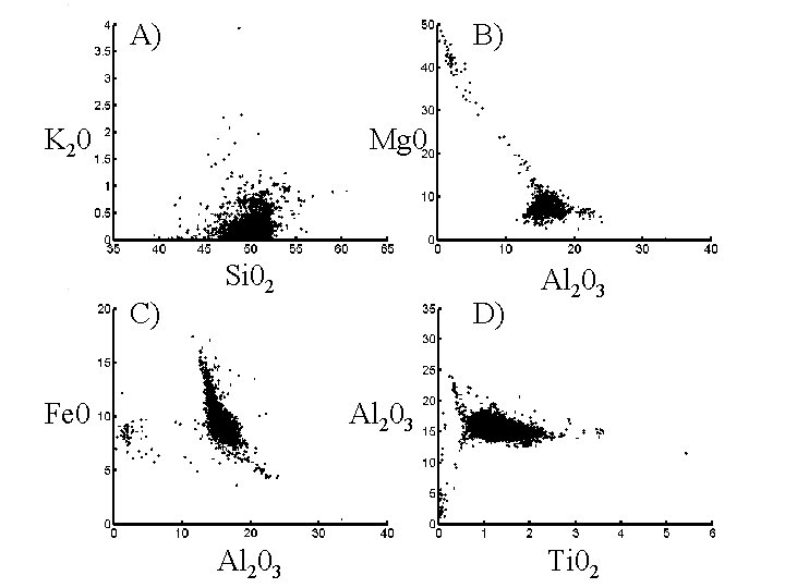
A) B) K 20 Mg 0 C) Si 02 Fe 0 D) Al 203 Ti 02
index, i singular values, λi
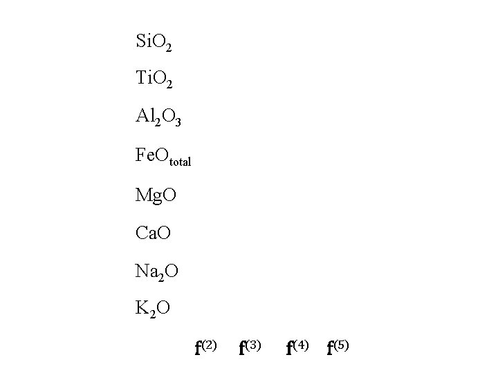
Si. O 2 Ti. O 2 Al 2 O 3 Fe. Ototal Mg. O Ca. O Na 2 O K 2 O f(2) f(3) f(4) f(5)
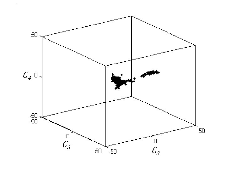
C 4 C 3 C 2
- Slides: 32