Lecture 16 Dataflow Analysis THEORY OF COMPILATION Eran

Lecture 16 – Dataflow Analysis THEORY OF COMPILATION Eran Yahav www. cs. technion. ac. il/~yahave/tocs 2011/compilers-lec 16. pptx Reference: Dragon 9, 12 1

Last time… Dataflow Analysis Information flows along (potential) execution paths Conservative approximation of all possible program executions Can be viewed as a sequence of transformations on program state Every statement (block) is associated with two abstract states: input state, output state Input/output state represents all possible states that can occur at the program point Representation is finite Different problems typically use different representations 2

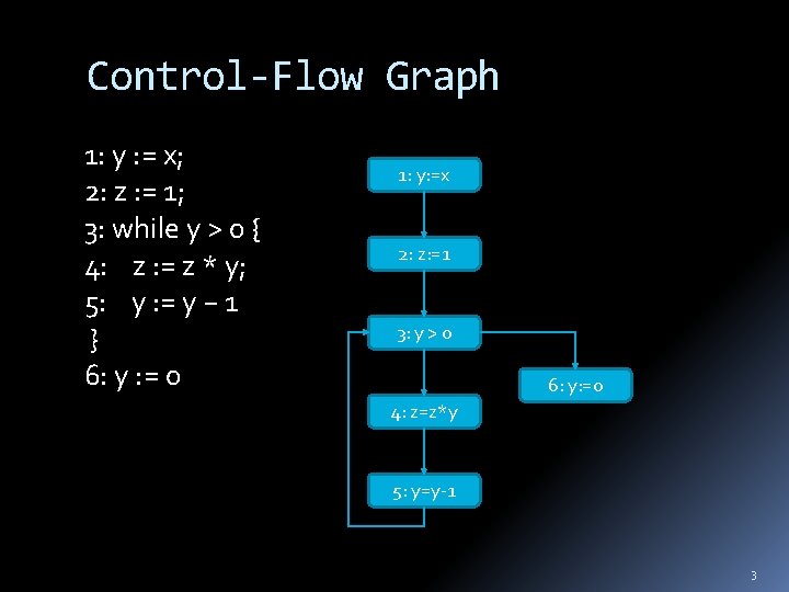
Control-Flow Graph 1: y : = x; 2: z : = 1; 3: while y > 0 { 4: z : = z * y; 5: y : = y − 1 } 6: y : = 0 1: y: =x 2: z: =1 3: y > 0 6: y: =0 4: z=z*y 5: y=y-1 3

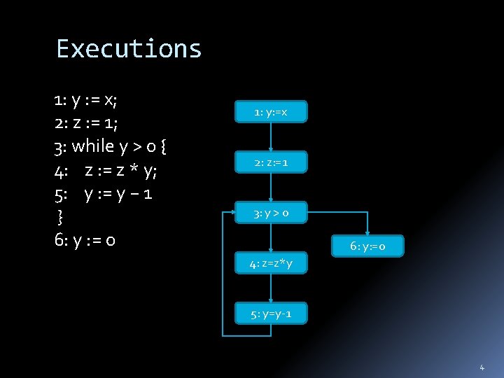
Executions 1: y : = x; 2: z : = 1; 3: while y > 0 { 4: z : = z * y; 5: y : = y − 1 } 6: y : = 0 1: y: =x 2: z: =1 3: y > 0 6: y: =0 4: z=z*y 5: y=y-1 4

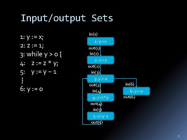
Input/output Sets 1: y : = x; 2: z : = 1; 3: while y > 0 { 4: z : = z * y; 5: y : = y − 1 } 6: y : = 0 in(1) 1: y: =x out(1) in(2) 2: z: =1 out(2) in(3) 3: y > 0 out(3) in(4) 4: z=z*y out(4) in(5) 5: y=y-1 out(5) in(6) 6: y: =0 out(6) 5

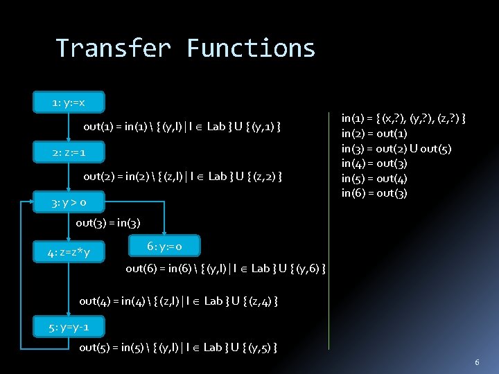
Transfer Functions 1: y: =x out(1) = in(1) { (y, l) | l Lab } U { (y, 1) } 2: z: =1 out(2) = in(2) { (z, l) | l Lab } U { (z, 2) } 3: y > 0 in(1) = { (x, ? ), (y, ? ), (z, ? ) } in(2) = out(1) in(3) = out(2) U out(5) in(4) = out(3) in(5) = out(4) in(6) = out(3) = in(3) 4: z=z*y 6: y: =0 out(6) = in(6) { (y, l) | l Lab } U { (y, 6) } out(4) = in(4) { (z, l) | l Lab } U { (z, 4) } 5: y=y-1 out(5) = in(5) { (y, l) | l Lab } U { (y, 5) } 6

Kill/Gen formulation for Reaching Definitions Block out (lab) [x : = a]lab in(lab) { (x, l) | l Lab } U { (x, lab) } [skip]lab in(lab) [b]lab in(lab) Block kill gen [x : = a]lab { (x, l) | l Lab } { (x, lab) } [skip]lab [b]lab For each program point, which assignments may have been made and not overwritten, when program execution reaches this point along some path. 7

Solving Gen/Kill Equations OUT[ENTRY] = ; for (each basic block B other than ENTRY) OUT[B] = ; while (changes to any OUT occur) { for (each basic block B other than ENTRY) { OUT[B]= (IN[B] kill. B) gen. B IN[B] = p pred(B) IN[p] } } Designated block Entry with OUT[Entry]= pred(B) = predecessor nodes of B in the control flow graph 8

Available Expressions Analysis [x : = a+b]1; [y : = a*b]2; while [y > a+b]3 ( [a : = a + 1]4; [x : = a + b]5 ) (a+b) always available at label 3 For each program point, which expressions must have already been computed, and not later modified, on all paths to the program point 9

Some required notation blocks : Stmt P(Blocks) blocks([x : = a]lab) = {[x : = a]lab} blocks([skip]lab) = {[skip]lab} blocks(S 1; S 2) = blocks(S 1) blocks(S 2) blocks(if [b]lab then S 1 else S 2) = {[b]lab} blocks(S 1) blocks(S 2) blocks(while [b]lab do S) = {[b]lab} blocks(S) FV: (BExp AExp) Variables used in an expression AExp(a) = all non-unit expressions in the arithmetic expression a similarly AExp(b) for a boolean expression b 10

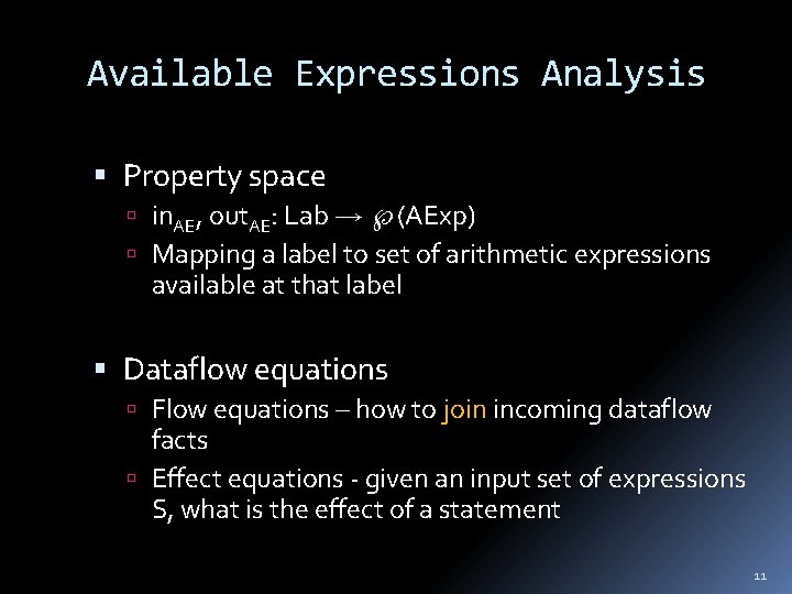
Available Expressions Analysis Property space in. AE, out. AE: Lab (AExp) Mapping a label to set of arithmetic expressions available at that label Dataflow equations Flow equations – how to join incoming dataflow facts Effect equations - given an input set of expressions S, what is the effect of a statement 11

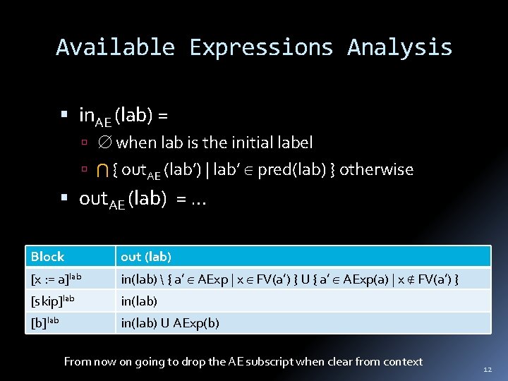
Available Expressions Analysis in. AE (lab) = when lab is the initial label { out. AE (lab’) | lab’ pred(lab) } otherwise out. AE (lab) = … Block out (lab) [x : = a]lab in(lab) { a’ AExp | x FV(a’) } U { a’ AExp(a) | x FV(a’) } [skip]lab in(lab) [b]lab in(lab) U AExp(b) From now on going to drop the AE subscript when clear from context 12

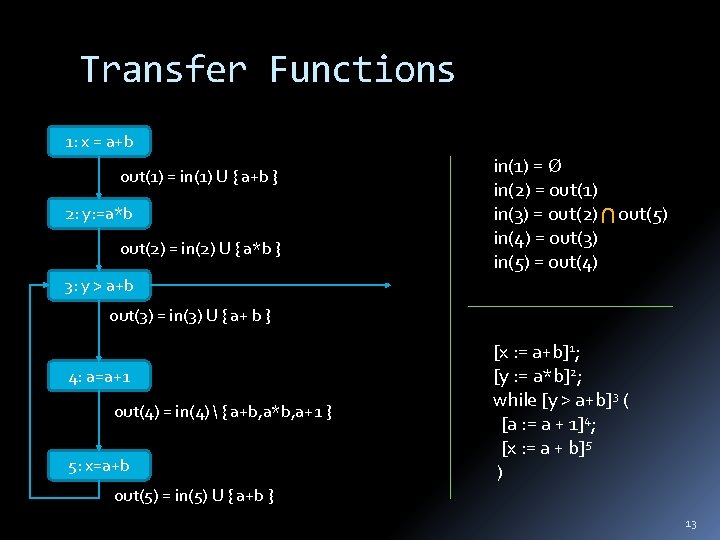
Transfer Functions 1: x = a+b out(1) = in(1) U { a+b } 2: y: =a*b out(2) = in(2) U { a*b } in(1) = in(2) = out(1) in(3) = out(2) out(5) in(4) = out(3) in(5) = out(4) 3: y > a+b out(3) = in(3) U { a+ b } 4: a=a+1 out(4) = in(4) { a+b, a*b, a+1 } 5: x=a+b [x : = a+b]1; [y : = a*b]2; while [y > a+b]3 ( [a : = a + 1]4; [x : = a + b]5 ) out(5) = in(5) U { a+b } 13

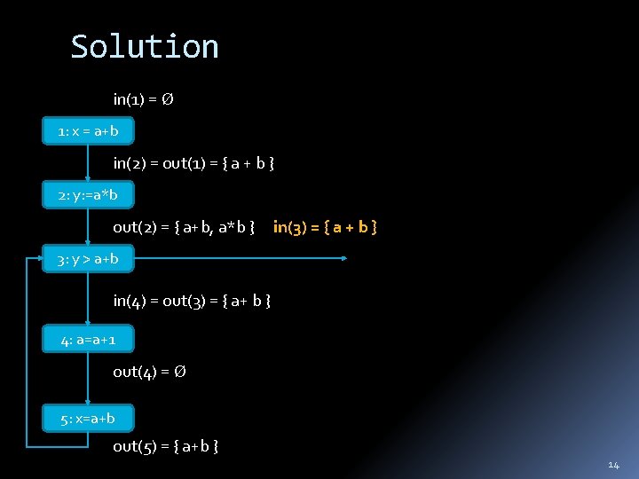
Solution in(1) = 1: x = a+b in(2) = out(1) = { a + b } 2: y: =a*b out(2) = { a+b, a*b } in(3) = { a + b } 3: y > a+b in(4) = out(3) = { a+ b } 4: a=a+1 out(4) = 5: x=a+b out(5) = { a+b } 14

Kill/Gen Block out (lab) [x : = a]lab in(lab) { a’ AExp | x FV(a’) } U { a’ AExp(a) | x FV(a’) } [skip]lab in(lab) [b]lab in(lab) U AExp(b) Block kill gen [x : = a]lab { a’ AExp | x FV(a’) } { a’ AExp(a) | x FV(a’) } [skip]lab [b]lab AExp(b) out(lab) = in(lab) kill(Blab) U gen(Blab) Blab = block at label lab 15

Reaching Definitions Revisited Block out (lab) [x : = a]lab in(lab) { (x, l) | l Lab } U { (x, lab) } [skip]lab in(lab) [b]lab in(lab) Block kill gen [x : = a]lab { (x, l) | l Lab } { (x, lab) } [skip]lab [b]lab For each program point, which assignments may have been made and not overwritten, when program execution reaches this point along some path. 16

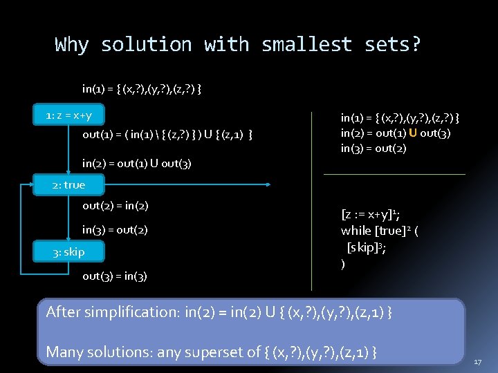
Why solution with smallest sets? in(1) = { (x, ? ), (y, ? ), (z, ? ) } 1: z = x+y out(1) = ( in(1) { (z, ? ) } ) U { (z, 1) } in(1) = { (x, ? ), (y, ? ), (z, ? ) } in(2) = out(1) U out(3) in(3) = out(2) in(2) = out(1) U out(3) 2: true out(2) = in(2) in(3) = out(2) 3: skip out(3) = in(3) [z : = x+y]1; while [true]2 ( [skip]3; ) After simplification: in(2) = in(2) U { (x, ? ), (y, ? ), (z, 1) } Many solutions: any superset of { (x, ? ), (y, ? ), (z, 1) } 17

Live Variables [x : =2]1; [y: =4]2; [x: =1]3; (if [y>x]4 then [z: =y]5 else [z: =y*y]6); [x: =z]7 For each program point, which variables may be live at the exit from the point. 18

Live Variables [x : =2]1; [y: =4]2; [x: =1]3; (if [y>x]4 then [z: =y]5 else [z: =y*y]6); [x: =z]7 1: x : = 2 2: y: =4 3: x: =1 4: y > x 5: z : = y 7: x : = z 6: z = y*y

Live Variables [x : =2]1; [y: =4]2; [x: =1]3; (if [y>x]4 then [z: =y]5 else [z: =y*y]6); [x: =z]7 Block kill gen {x} { FV(a) } [skip]lab [b]lab FV(b) [x : = a]lab 1: x : = 2 2: y: =4 3: x: =1 4: y > x 5: z : = y 6: z = y*y 7: x : = z 20

Live Variables: solution in(1) = [x : =2]1; [y: =4]2; [x: =1]3; (if [y>x]4 then [z: =y]5 else [z: =y*y]6); [x: =z]7 Block kill gen {x} { FV(a) } [skip]lab [b]lab FV(b) [x : = a]lab 1: x : = 2 out(1) = in(2) = 2: y: =4 out(2) = in(3) = { y } 3: x: =1 out(3) = in(4) = { x, y } 4: y > x out(4) = { y } in(5) = { y } 5: z : = y out(5) = { z } in(7) = { z } in(6) = { y } 6: z = y*y out(6) = { z } 7: x : = z out(7) = 21

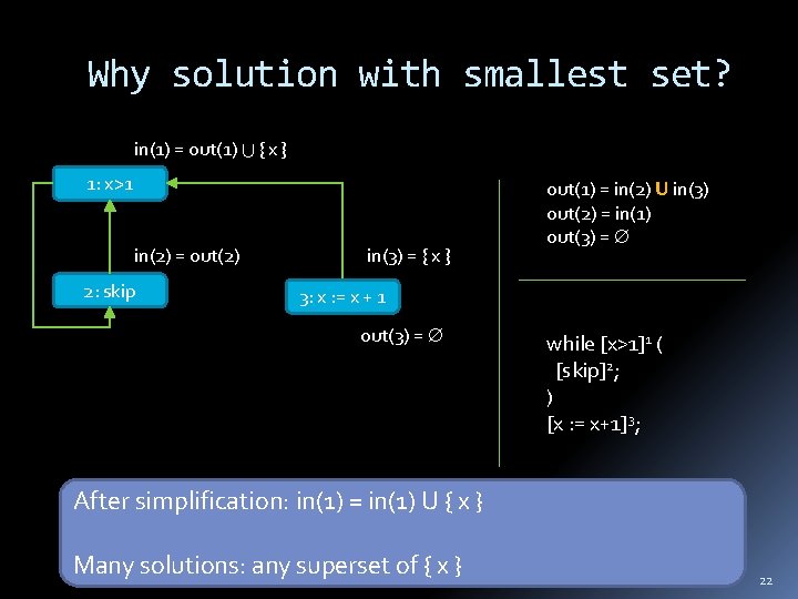
Why solution with smallest set? in(1) = out(1) { x } 1: x>1 in(2) = out(2) 2: skip in(3) = { x } out(1) = in(2) U in(3) out(2) = in(1) out(3) = 3: x : = x + 1 out(3) = while [x>1]1 ( [skip]2; ) [x : = x+1]3; After simplification: in(1) = in(1) U { x } Many solutions: any superset of { x } 22

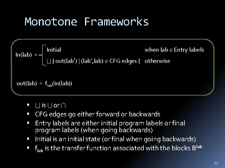
Monotone Frameworks In(lab) = Initial when lab Entry labels { out(lab’) | (lab’, lab) CFG edges } otherwise out(lab) = flab(in(lab)) is or CFG edges go either forward or backwards Entry labels are either initial program labels or final program labels (when going backwards) Initial is an initial state (or final when going backwards) flab is the transfer function associated with the blocks Blab 23

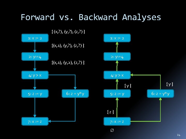
Forward vs. Backward Analyses { (x, ? ), (y, ? ), (z, ? ) } 1: x : = 2 {(x, 1), (y, ? ), (z, ? ) } 2: y: =4 {(x, 1), (y, 2), (z, ? ) } 4: y > x {y} 5: z : = y 6: z = y*y 5: z : = y {y} 6: z = y*y {z} 7: x : = z 24

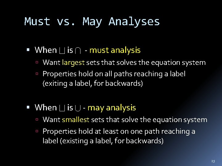
Must vs. May Analyses When is - must analysis Want largest sets that solves the equation system Properties hold on all paths reaching a label (exiting a label, for backwards) When is - may analysis Want smallest sets that solve the equation system Properties hold at least on one path reaching a label (existing a label, for backwards) 25

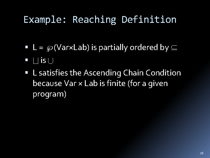
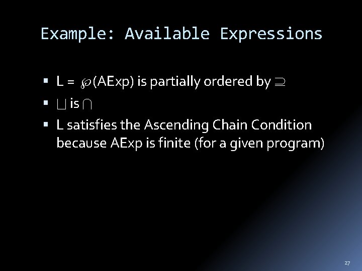
Example: Reaching Definition L = (Var×Lab) is partially ordered by is L satisfies the Ascending Chain Condition because Var × Lab is finite (for a given program) 26

Example: Available Expressions L = (AExp) is partially ordered by is L satisfies the Ascending Chain Condition because AExp is finite (for a given program) 27

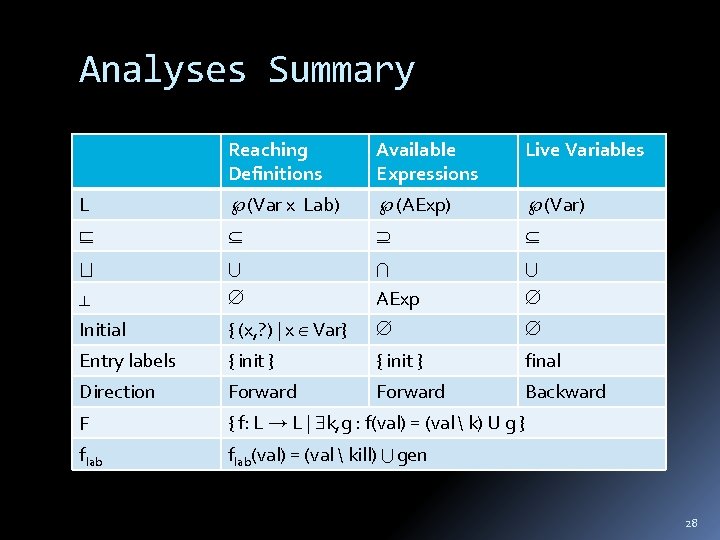
Analyses Summary Reaching Definitions Available Expressions Live Variables L (Var x Lab) (AExp) (Var) AExp Initial { (x, ? ) | x Var} Entry labels { init } final Direction Forward Backward F { f: L L | k, g : f(val) = (val k) U g } flab(val) = (val kill) gen 28

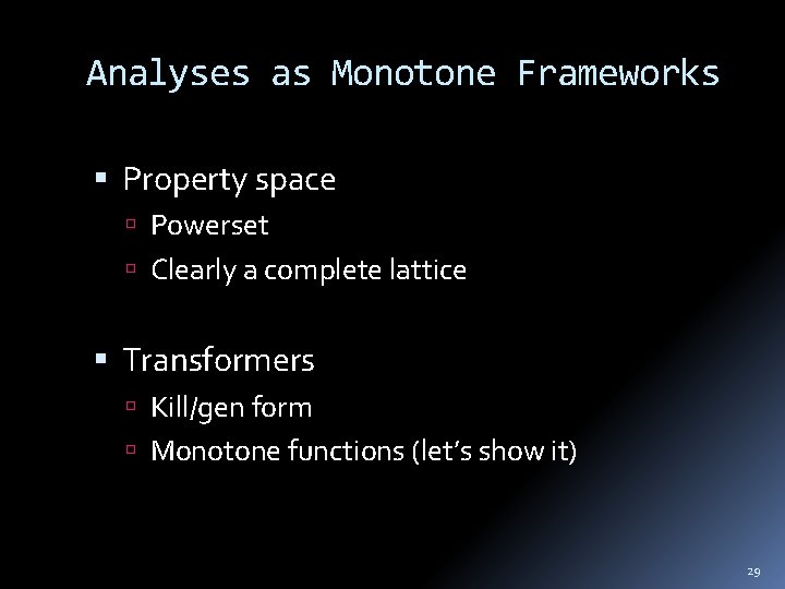
Analyses as Monotone Frameworks Property space Powerset Clearly a complete lattice Transformers Kill/gen form Monotone functions (let’s show it) 29

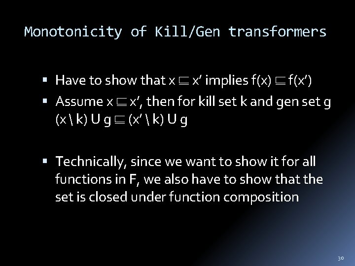
Monotonicity of Kill/Gen transformers Have to show that x x’ implies f(x) f(x’) Assume x x’, then for kill set k and gen set g (x k) U g (x’ k) U g Technically, since we want to show it for all functions in F, we also have to show that the set is closed under function composition 30

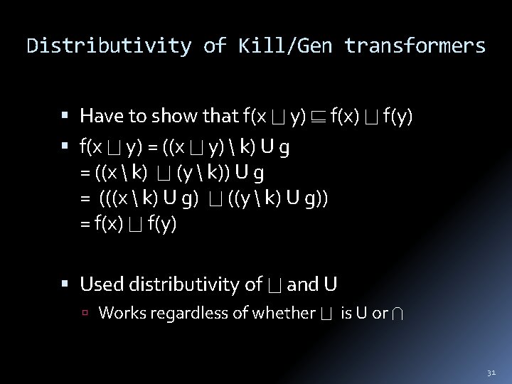
Distributivity of Kill/Gen transformers Have to show that f(x y) f(x) f(y) f(x y) = ((x y) k) U g = ((x k) (y k)) U g = (((x k) U g) ((y k) U g)) = f(x) f(y) Used distributivity of and U Works regardless of whether is U or 31

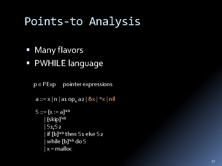
Points-to Analysis Many flavors PWHILE language p PExp pointer expressions a : : = x | n | a 1 opa a 2 | &x | *x | nil S : : = [x : = a]lab | [skip]lab | S 1; S 2 | if [b]lab then S 1 else S 2 | while [b]lab do S | x = malloc 32

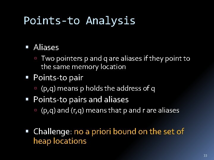
Points-to Analysis Aliases Two pointers p and q are aliases if they point to the same memory location Points-to pair (p, q) means p holds the address of q Points-to pairs and aliases (p, q) and (r, q) means that p and r are aliases Challenge: no a priori bound on the set of heap locations 33

Terminology Example [x : = &z]1 [y : = &z]2 [w : = &y]3 [r : = w]4 x z y r w Points-to pairs: (x, z), (y, z), (w, y), (r, y) Aliases: (x, y), (r, w) 34

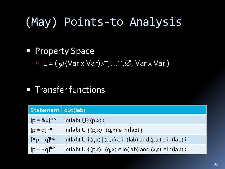
(May) Points-to Analysis Property Space L = ( (Var x Var), , , Var x Var ) Transfer functions Statement out(lab) [p = &x]lab in(lab) { (p, x) } [p = q]lab in(lab) U { (p, x) | (q, x) in(lab) } [*p = q]lab in(lab) U { (r, x) | (q, x) in(lab) and (p, r) in(lab) } [p = *q]lab in(lab) U { (p, r) | (q, x) in(lab) and (x, r) in(lab) } 35

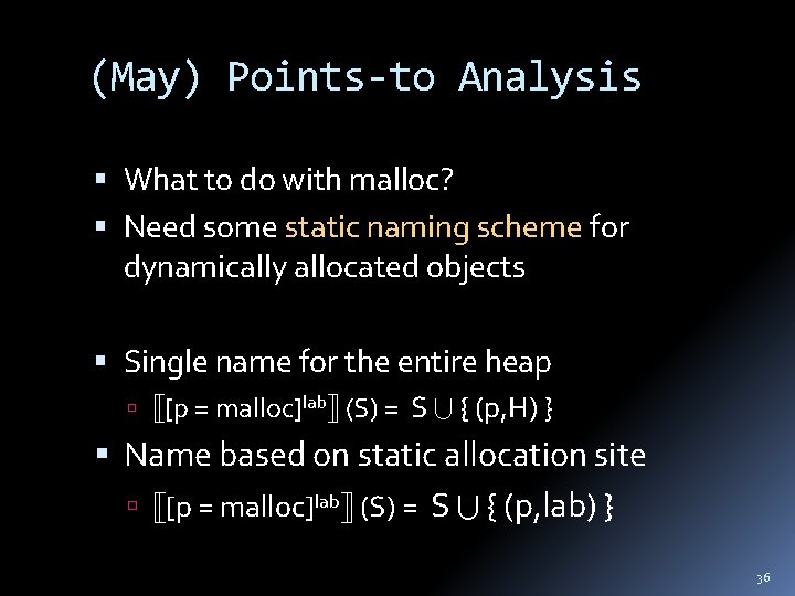
(May) Points-to Analysis What to do with malloc? Need some static naming scheme for dynamically allocated objects Single name for the entire heap [p = malloc]lab (S) = S { (p, H) } Name based on static allocation site [p = malloc]lab (S) = S { (p, lab) } 36

(May) Points-to Analysis [x : =malloc]1; [y: =malloc]2; (if [x==y]3 then [z: =x]4 else [z: =y]5 ); { (x, H) } { (x, H), (y, H), (z, H) } { (x, H), (y, H), (z, H) } Single name H for the entire heap 37

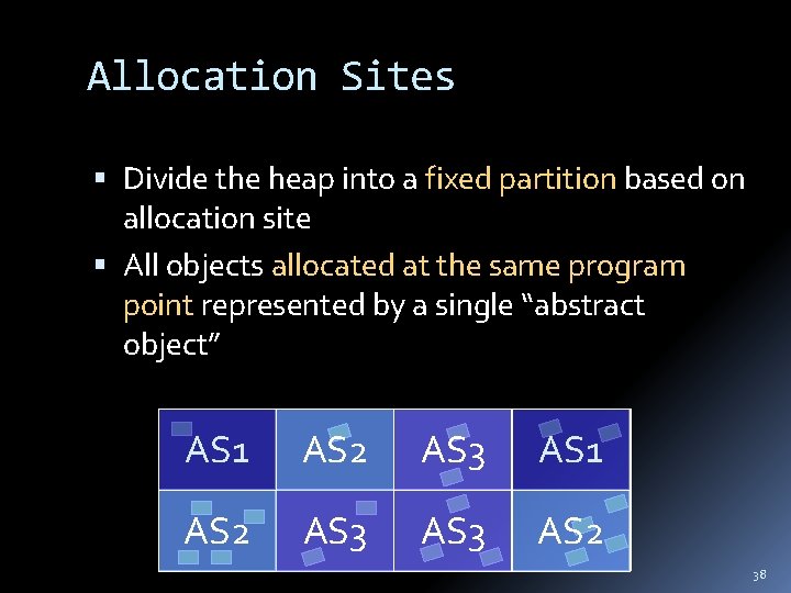
Allocation Sites Divide the heap into a fixed partition based on allocation site All objects allocated at the same program point represented by a single “abstract object” AS 1 AS 2 AS 3 AS 2 38

(May) Points-to Analysis [x : =malloc]1; // A 1 [y: =malloc]2; // A 2 (if [x==y]3 then [z: =x]4 else [z: =y]5 ); { (x, A 1) } { (x, A 1), (y, A 2), (z, A 1) } { (x, A 1), (y, A 2), (z, A 2) } { (x, A 1), (y, A 2), (z, A 1), (z, A 2) } Allocation-site based naming (using Alab instead of just “lab” for clarity) 39

Weak Updates Statement out(lab) [p = &x]lab in(lab) { (p, x) } [p = q]lab in(lab) U { (p, x) | (q, x) in(lab) } [*p = q]lab in(lab) U { (r, x) | (q, x) in(lab) and (p, r) in(lab) } [p = *q]lab in(lab) U { (p, r) | (q, x) in(lab) and (x, r) in(lab) } [x : =malloc]1; // A 1 [y: =malloc]2; // A 2 [z: =x]3; [z: =y]4; { (x, A 1) } { (x, A 1), (y, A 2), (z, A 1), (z, A 2) } 40

(May) Points-to Analysis Fixed partition of the (unbounded) heap to static names Allocation sites Types Calling contexts … What we saw so far – flow-insensitive Ignoring the structure of the flow in the program 41

Flow-sensitive vs. Flow-insensitive Analyses [x : =malloc]1; [y: =malloc]2; (if [x==y]3 then [z: =x]4 else [z: =y]5 ); 1: x : = malloc 2: y: =malloc 3: x == y 4: z : = x 6: z = y Flow sensitive: respect program flow a separate set of points-to pairs for every program point the set at a point represents possible may-aliases on some path from entry to the program point Flow insensitive: assume all execution orders are possible, abstract away order between statements 42

So far… Intra-procedural analysis How are we going to deal with procedures? Inter-procedural analysis 43

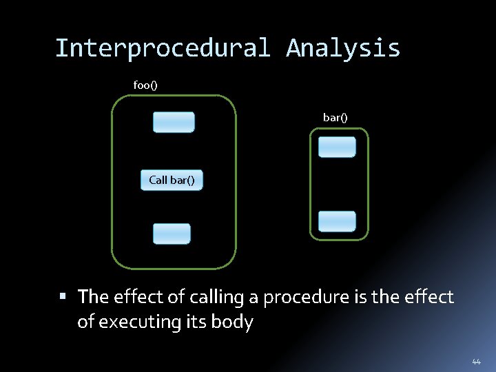
Interprocedural Analysis foo() bar() Call bar() The effect of calling a procedure is the effect of executing its body 44

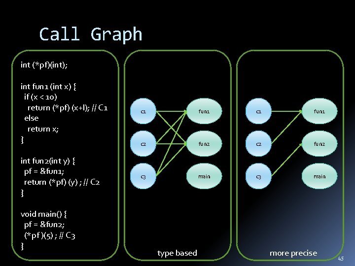
Call Graph int (*pf)(int); int fun 1 (int x) { if (x < 10) return (*pf) (x+l); // C 1 else return x; } int fun 2(int y) { pf = &fun 1; return (*pf) (y) ; // C 2 } void main() { pf = &fun 2; (*pf )(5) ; // C 3 } c 1 fun 1 c 2 fun 2 c 3 main type based more precise 45

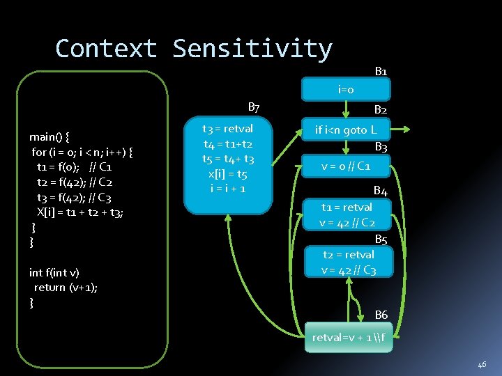
Context Sensitivity B 1 i=0 B 7 main() { for (i = 0; i < n; i++) { t 1 = f(0); // C 1 t 2 = f(42); // C 2 t 3 = f(42); // C 3 X[i] = t 1 + t 2 + t 3; } } int f(int v) return (v+1); } t 3 = retval t 4 = t 1+t 2 t 5 = t 4+ t 3 x[i] = t 5 i=i+1 B 2 if i<n goto L B 3 v = 0 // C 1 B 4 t 1 = retval v = 42 // C 2 B 5 t 2 = retval v = 42 // C 3 B 6 retval=v + 1 \f 46

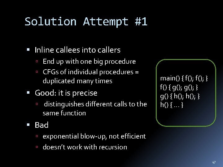
Solution Attempt #1 Inline callees into callers End up with one big procedure CFGs of individual procedures = duplicated many times Good: it is precise distinguishes different calls to the same function main() { f(); } f() { g(); } g() { h(); } h() {. . . } Bad exponential blow-up, not efficient doesn’t work with recursion 47

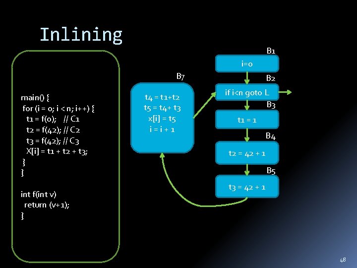
Inlining B 1 i=0 B 7 main() { for (i = 0; i < n; i++) { t 1 = f(0); // C 1 t 2 = f(42); // C 2 t 3 = f(42); // C 3 X[i] = t 1 + t 2 + t 3; } } int f(int v) return (v+1); } t 4 = t 1+t 2 t 5 = t 4+ t 3 x[i] = t 5 i=i+1 B 2 if i<n goto L B 3 t 1 = 1 B 4 t 2 = 42 + 1 B 5 t 3 = 42 + 1 48

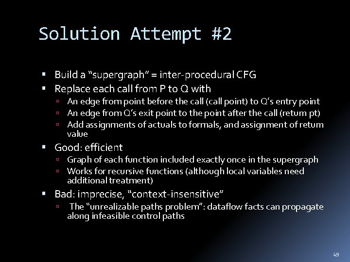
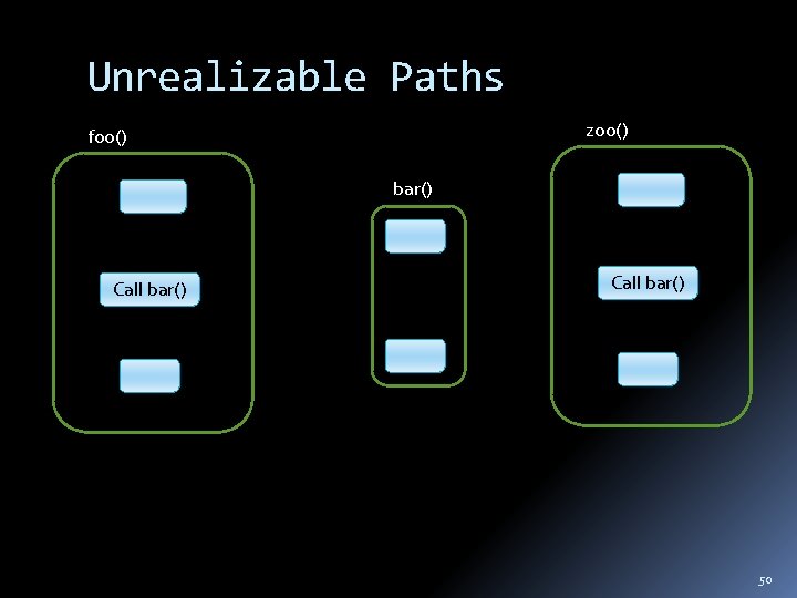
Solution Attempt #2 Build a “supergraph” = inter-procedural CFG Replace each call from P to Q with An edge from point before the call (call point) to Q’s entry point An edge from Q’s exit point to the point after the call (return pt) Add assignments of actuals to formals, and assignment of return value Good: efficient Graph of each function included exactly once in the supergraph Works for recursive functions (although local variables need additional treatment) Bad: imprecise, “context-insensitive” The “unrealizable paths problem”: dataflow facts can propagate along infeasible control paths 49

Unrealizable Paths zoo() foo() bar() Call bar() 50

Interprocedural Analysis begin proc p() is 1 [x : = a + 1]2 end 3 [a=7]4 [call p()]56 [print x]7 [a=9]8 [call p()]910 [print a]11 end Extend language with begin/end and with [call p()]clabrlab Call label clab, and return label rlab 51

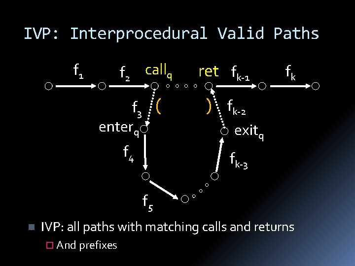
IVP: Interprocedural Valid Paths f 2 callq f 1 f 3 ( enterq f 4 ret fk-1 ) fk fk-2 exitq fk-3 f 5 n IVP: all paths with matching calls and returns ¨ And prefixes

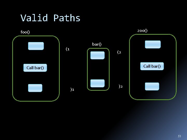
Valid Paths zoo() foo() bar() (1 (2 Call bar() )1 )2 53

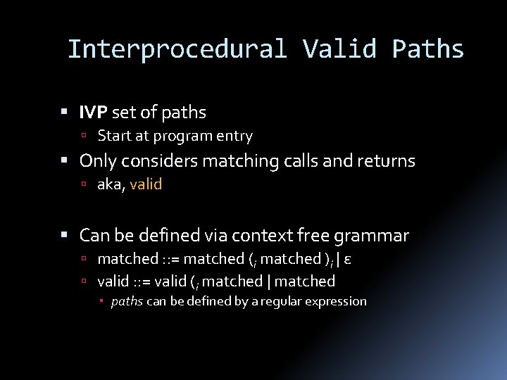
Interprocedural Valid Paths IVP set of paths Start at program entry Only considers matching calls and returns aka, valid Can be defined via context free grammar matched : : = matched (i matched )i | ε valid : : = valid (i matched | matched paths can be defined by a regular expression

The Join-Over-Valid-Paths (JVP) vpaths(n) all valid paths from program start to n JVP[n] = { e 1, e 2, …, e (initial) (e 1, e 2, …, e) vpaths(n)} JVP JFP In some cases the JVP can be computed (Distributive problem)

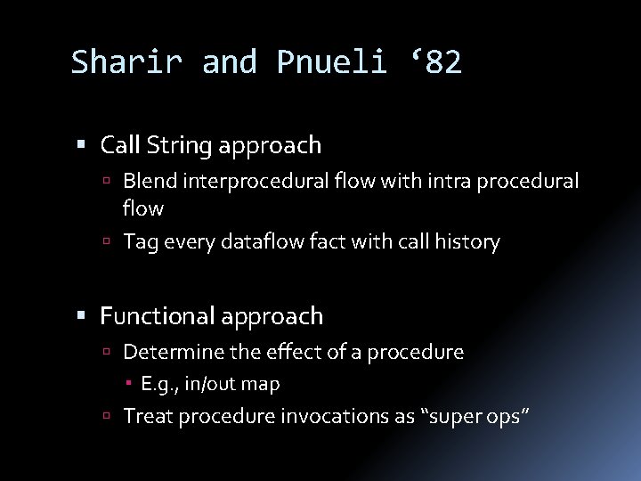
Sharir and Pnueli ‘ 82 Call String approach Blend interprocedural flow with intra procedural flow Tag every dataflow fact with call history Functional approach Determine the effect of a procedure E. g. , in/out map Treat procedure invocations as “super ops”

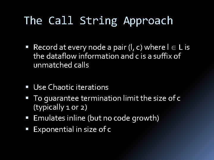
The Call String Approach Record at every node a pair (l, c) where l L is the dataflow information and c is a suffix of unmatched calls Use Chaotic iterations To guarantee termination limit the size of c (typically 1 or 2) Emulates inline (but no code growth) Exponential in size of c

[x 0, a 0] begin proc p() is 1 [x : = a + 1]2 end 3 [x 0, a 7] call p 5 [x 8, a 7] [a=7]4 [x 8, a 7] [call p()]56 [x 8, a 7] [print x]7 [a=9]8 [call p()]910 [print a]11 end a=7 [x 8, a 9] call p 6 print x 9, [x 8, a 9] 5, [x 0, a 7] x=a+1 9, [x 10, a 9] 5, [x 8, a 7] end 9, [x 10, a 9] 5, [x 8, a 7] proc p a=9 call p 10 print a [x 10, a 9]

10: [x 0, a 7] 4: [x 0, a 6] begin 0 p proc p() is 1 if [b]2 [x 0, a 0] then ( [a : = a -1]3 [x 0, a 7] [call p()]45 [a : = a + 1]6 ) [x : = -2* a + 5]7 a=7 Call p 10 Call print(x) end 8 [a=7]9 ; [call p()]1011 ; [print(x)]12 end 13 p 11 10: [x 0, a 7] a=a-1 10: [x 0, a 6] Call p 4 Call p 5 a=a+1 4: [x -7, a 7] If( … ) 10: [x -7, a 6] 4: [x 0, a 6] 4: [x , a ] 4: [x -7, a 6] x=-2 a+5 end

The Functional Approach The meaning of a procedure is mapping from states into states The abstract meaning of a procedure is function from an abstract state to abstract states

e. [x -2 e(a)+5, a e(a)] begin p proc p() is 1 if [b]2 [x 0, a 0] then ( [a : = a -1]3 [x 0, a 7] Call p 10 [call p()]45 [a : = a + 1]6 [x -9, a 7] ) a=7 Call p 11 [x -9, a 7] [x : = -2* a + 5]7 print(x) end 8 [a=7]9 ; [call p()]1011 ; [print(x)]12 end If( … ) a=a-1 Call p 4 Call p 5 a=a+1 x=-2 a+5 end

e. [x -2 e(a)+5, a e(a)] begin p proc p() is 1 if [b]2 [x 0, a 0] then ( [a : = a -1]3 [x 0, a ] Call p 10 [call p()]45 [a : = a + 1]6 [x , a ] ) read(a) Call p 11 [x , a ] [x : = -2* a + 5]7 print(x) end 8 [read(a)]9 ; [call p()]1011 ; [print(x)]12 end If( … ) a=a-1 Call p 4 Call p 5 a=a+1 x=-2 a+5 end

Functional Approach: Main Idea Iterate on the abstract domain of functions from L to L Two phase algorithm Compute the dataflow solution at the exit of a procedure as a function of the initial values at the procedure entry (functional values) Compute the dataflow values at every point using the functional values Computes JVP for distributive problems