Lecture 16 Basic properties of Fourier Transforms Mat

Lecture 16 Basic properties of Fourier Transforms

Mat. Lab Code % setup N=256; dt=1. 0; tmax=dt*(N-1); t=dt*[0: N-1]; fmax=1/(2. 0*dt); df=fmax/(N/2); f=df*[0: N/2, -N/2+1: -1]'; dw=2*pi*df; w=dw*[0: N/2, -N/2+1: -1]'; % a sample function, p(t) w 0 = 2*pi*fmax/10; p = sin(w 0*t). *exp(-0. 25*w 0*t); pt=fft(p); % fourier transform pr=ifft(pt); % inverse transform

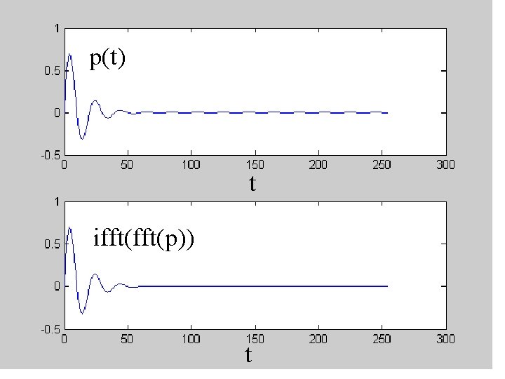
p(t) t ifft(p)) t

1: Relationship to integral transforms Integral transforms: + C(w) = - T(t) exp(-iwt) dt + T(t) = (1/2 p) - C(w) exp(iwt) dw Discrete transforms Ck = Sn=-N/2 N/2 Tn exp(-2 pikn/N ) with k=-½N, …, ½N Tn = N-1 Sk=-N/2 N/2 Ck exp(+2 pikn/N ) with n=-½N, …, ½N (this agrees with definition in Mat. Lab HELP)

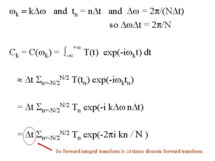
wk = k. Dw and tn = n. Dt and Dw = 2 p/(NDt) so Dw. Dt = 2 p/N Ck = C(wk) = - + T(t) exp(-iwkt) dt Dt Sn=-N/2 N/2 T(tn) exp(-iwktn) = Dt Sn=-N/2 N/2 Tn exp(-i k. Dw n. Dt) = Dt Sn=-N/2 N/2 Tn exp(-2 pi kn / N ) So forward integral transform is Dt times discrete forward transform

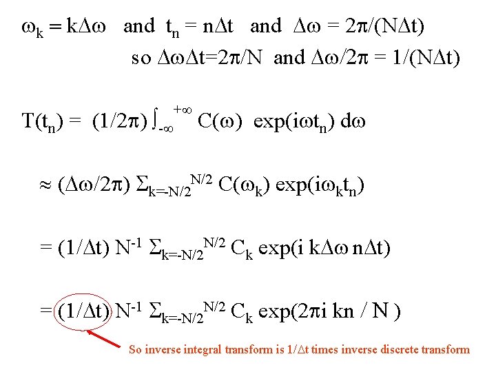
wk = k. Dw and tn = n. Dt and Dw = 2 p/(NDt) so Dw. Dt=2 p/N and Dw/2 p = 1/(NDt) T(tn) = (1/2 p) - + C(w) exp(iwtn) dw (Dw/2 p) Sk=-N/2 N/2 C(wk) exp(iwktn) = (1/Dt) N-1 Sk=-N/2 N/2 Ck exp(i k. Dw n. Dt) = (1/Dt) N-1 Sk=-N/2 N/2 Ck exp(2 pi kn / N ) So inverse integral transform is 1/Dt times inverse discrete transform

So … Except for a normalization factor of Dt, The discrete transform is just the “Riemann Sum” approximation to the integral transform, with particular choice Dw. Dt=2 p/N Properties of the integral transform carry over to the discrete transform (well, more-or-less)

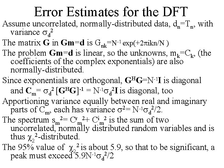
Error Estimates for the DFT Assume uncorrelated, normally-distributed data, dn=Tn, with variance sd 2 The matrix G in Gm=d is Gnk=N-1 exp(+2 pikn/N ) The problem Gm=d is linear, so the unknowns, mk=Ck, (the coefficients of the complex exponentials) are also normally-distributed. Since exponentials are orthogonal, GHG=N-1 I is diagonal and Cm= sd 2 [GHG]-1 = N-1 sd 2 I is diagonal, too Apportioning variance equally between real and imaginary parts of Cm, each has variance s 2= N-1 sd 2/2. The spectrum sm 2= Crm 2+ Cim 2 is the sum of two uncorrelated, normally distributed random variables and is thus c 22 -distributed. The 95% value of c 22 is about 5. 9, so that to be significant, a peak must exceed 5. 9 N-1 sd 2/2

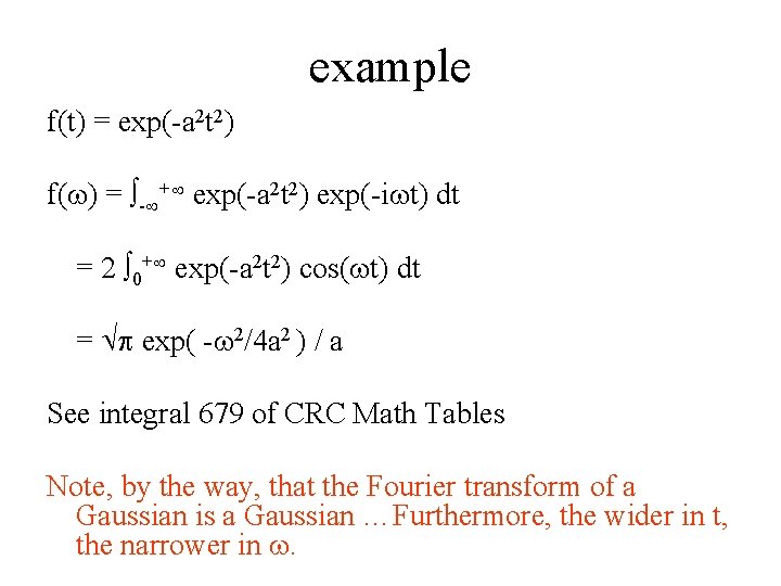
example f(t) = exp(-a 2 t 2) f(w) = - + exp(-a 2 t 2) exp(-iwt) dt = 2 0+ exp(-a 2 t 2) cos(wt) dt = p exp( -w 2/4 a 2 ) / a See integral 679 of CRC Math Tables Note, by the way, that the Fourier transform of a Gaussian is a Gaussian …Furthermore, the wider in t, the narrower in w.

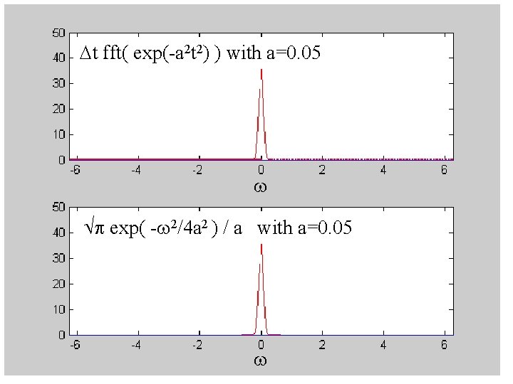
Dt fft( exp(-a 2 t 2) ) with a=0. 05 w p exp( -w 2/4 a 2 ) / a with a=0. 05 w

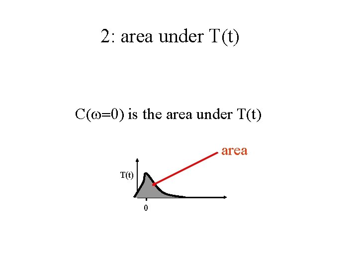
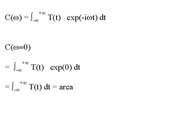
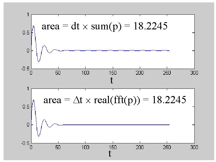
2: area under T(t) C(w=0) is the area under T(t) area T(t) 0

C(w) = - + T(t) exp(-iwt) dt C(w=0) = - + + T(t) exp(0) dt T(t) dt = area

area = dt sum(p) = 18. 2245 t area = Dt real(fft(p)) = 18. 2245 t

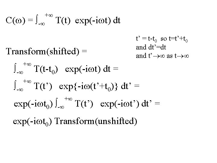
3: Time shift Multiplying C(w) by exp(-iwt 0) shifts the timeseries T(t) by t 0. T(t) T(t-t 0) 0 t 0

C(w) = - + T(t) exp(-iwt) dt Transform(shifted) = t’ = t-t 0 so t=t’+t 0 and dt’=dt and t’ as t - + T(t-t 0) exp(-iwt) dt = - + T(t’) exp{-iw(t’+t 0)} dt’ = exp(-iwt 0) - + T(t’) exp(-iwt’) dt’ = exp(-iwt 0) Transform(unshifted)

p(t) t ifft(exp(-iwt 0) fft(p(t))) with t 0=50 t

4: derivative Multiplying C(w) by iw Gives the transform of d. T/dt

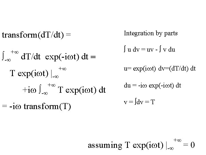
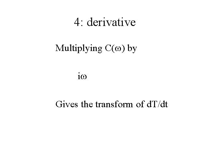
Integration by parts transform(d. T/dt) = - + d. T/dt exp(-iwt) dt = + u= exp(iwt) dv=(d. T/dt) dt T exp(iwt) dt du = -iw exp(-iwt) dt T exp(iwt) |- +iw - + u dv = uv - v du = -iw transform(T) v = dv = T assuming T exp(iwt) |- + =0

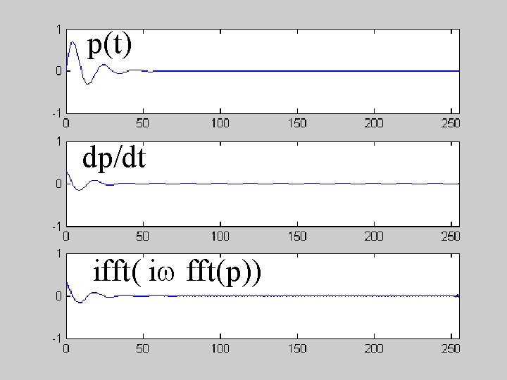
p(t) dp/dt ifft( iw fft(p))

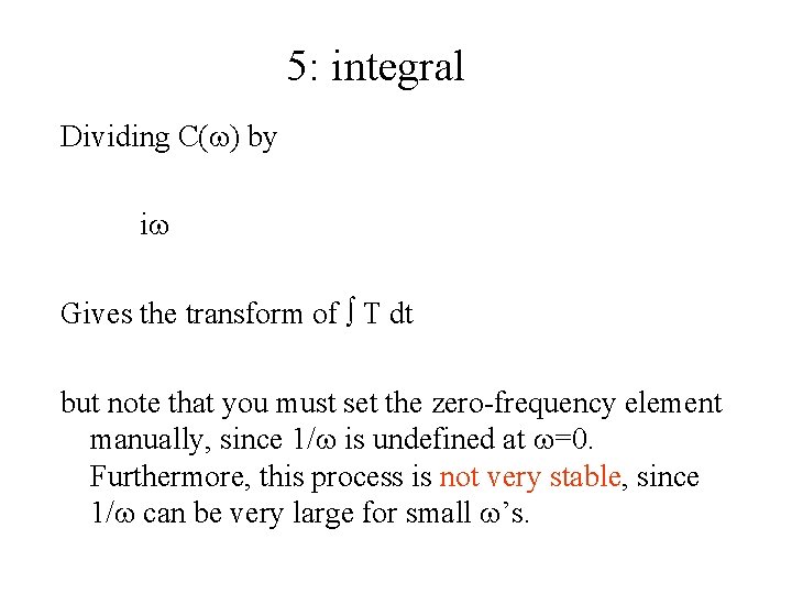
5: integral Dividing C(w) by iw Gives the transform of T dt but note that you must set the zero-frequency element manually, since 1/w is undefined at w=0. Furthermore, this process is not very stable, since 1/w can be very large for small w’s.

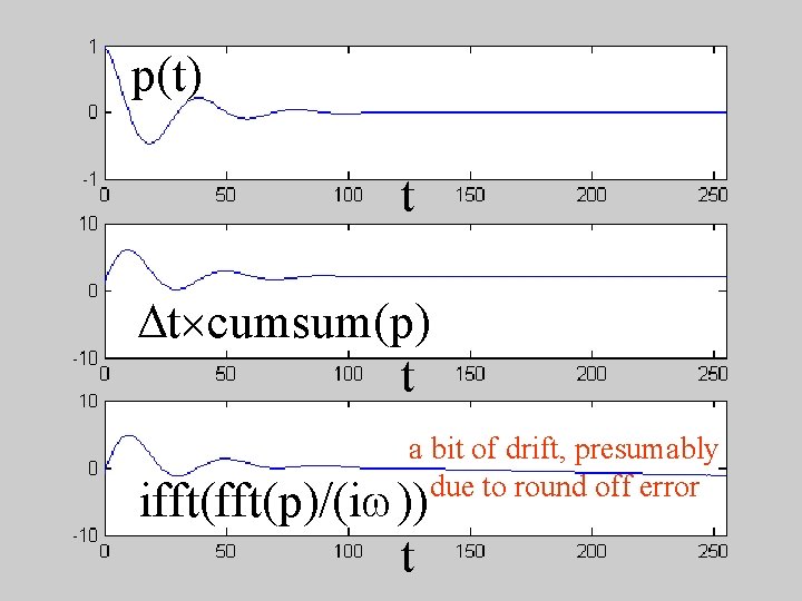
p(t) t Dt cumsum(p) t a bit of drift, presumably due to round off error ifft(p)/(iw)) t

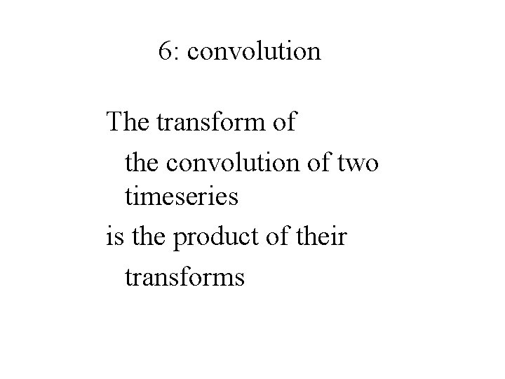
6: convolution The transform of the convolution of two timeseries is the product of their transforms

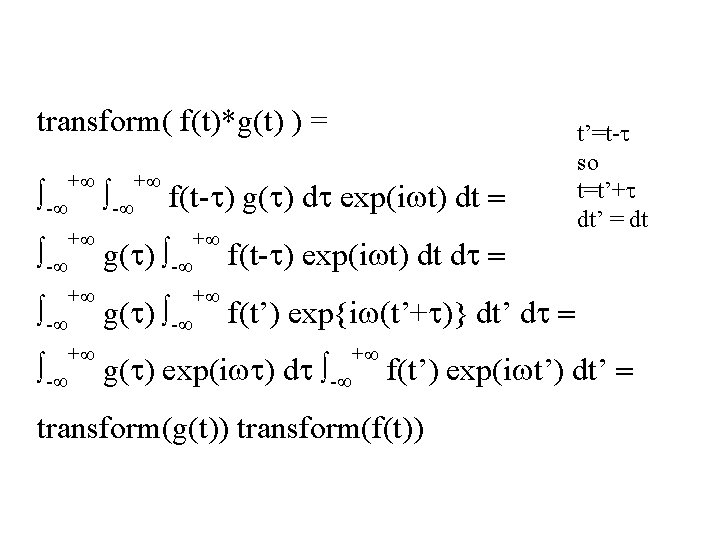
transform( f(t)*g(t) ) = - + - + f(t-t) g(t) dt exp(iwt) dt = g(t) - + f(t-t) exp(iwt) dt dt = g(t) - + f(t’) exp{iw(t’+t)} dt’ dt = g(t) exp(iwt) dt - + t’=t-t so t=t’+t dt’ = dt f(t’) exp(iwt’) dt’ = transform(g(t)) transform(f(t))

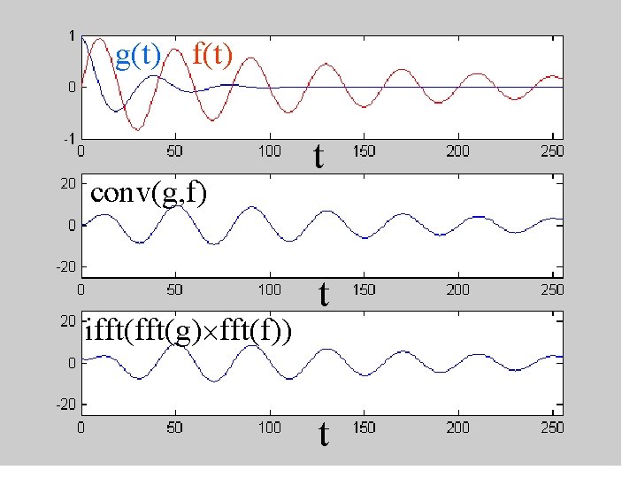
g(t) f(t) conv(g, f) ifft(g) fft(f)) t t t

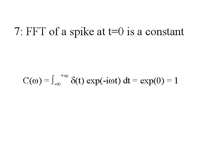
7: FFT of a spike at t=0 is a constant C(w) = - + d(t) exp(-iwt) dt = exp(0) = 1

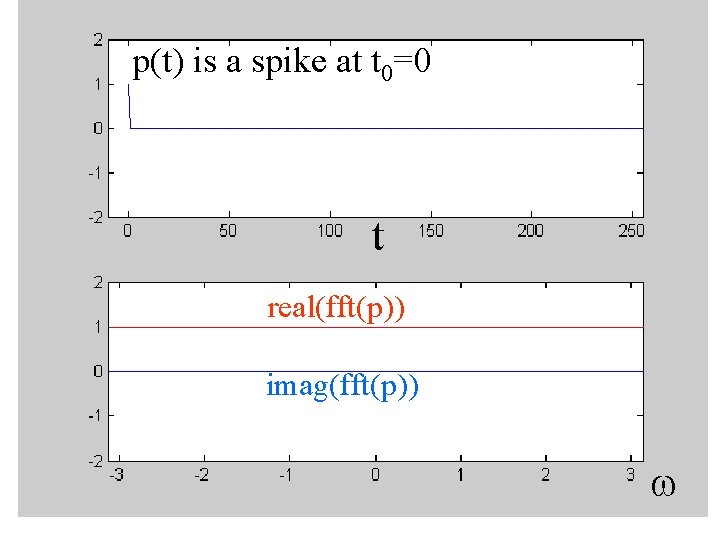
p(t) is a spike at t 0=0 t real(fft(p)) imag(fft(p)) w

7: FFT of a spike at t=t 0 is sinusoidal C(w) = - + d(t-t 0) exp(-iwt) dt = exp(-iwt 0) = cos(wt 0) - i sin(wt 0)

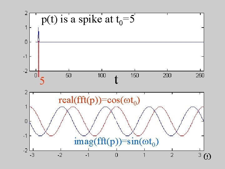
p(t) is a spike at t 0=5 5 t real(fft(p))=cos(wt 0) imag(fft(p))=sin(wt 0) w

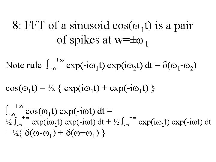
8: FFT of a sinusoid cos(w 1 t) is a pair of spikes at w=±w 1 Note rule - + exp(-iw 1 t) exp(iw 2 t) dt = d(w 1 -w 2) cos(w 1 t) = ½ { exp(iw 1 t) + exp(-iw 1 t) } - + cos(w 1 t) exp(-iwt) dt = + ½ - exp(iw 1 t) exp(-iwt) dt + ½ - = ½{ d(w-w 1) + d(w+w 1) } + exp(iw 1 t) exp(-iwt) dt

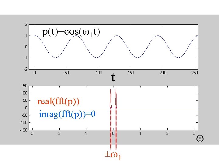
p(t)=cos(w 1 t) t real(fft(p)) imag(fft(p))=0 w ±w 1

Aliasing the tendency in a digital world for high frequencies to look like low frequencies

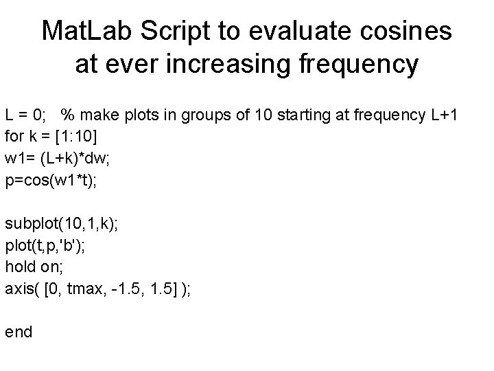
Mat. Lab Script to evaluate cosines at ever increasing frequency L = 0; % make plots in groups of 10 starting at frequency L+1 for k = [1: 10] w 1= (L+k)*dw; p=cos(w 1*t); subplot(10, 1, k); plot(t, p, 'b'); hold on; axis( [0, tmax, -1. 5, 1. 5] ); end

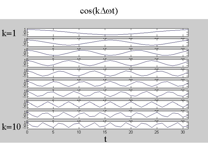
cos(k. Dwt) k=10 t

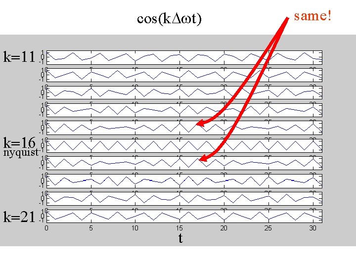
cos(k. Dwt) k=11 k=16 nyquist k=21 t same!

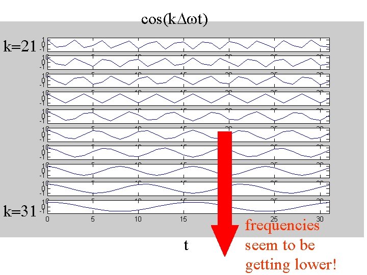
cos(k. Dwt) k=21 k=31 t frequencies seem to be getting lower!

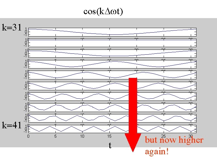
cos(k. Dwt) k=31 k=41 t but now higher again!

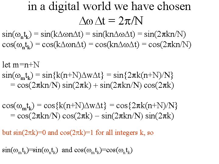
in a digital world we have chosen Dw. Dt = 2 p/N sin(wntk) = sin(k. Dwn. Dt) = sin(kn. Dw. Dt) = sin(2 pkn/N) cos(wntk) = cos(k. Dwn. Dt) = cos(kn. Dw. Dt) = cos(2 pkn/N) let m=n+N sin(wmtk) = sin{k(n+N)Dw. Dt} = sin{2 pk(n+N)/N} = cos(2 pkn/N) sin(2 pk) + sin(2 pkn/N) cos(2 pk) cos(wmtk) = cos{k(n+N)Dw. Dt} = cos{2 pk(n+N)/N} = cos(2 pkn/N) cos(2 pk) - sin(2 pkn/N) sin(2 pk) but sin(2 pk)=0 and cos(2 pk)=1 for all integers k, so sin(wmtk)=sin(wntk) and cos(wmtk)=cos(wntk)

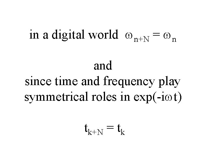
in a digital world wn+N = wn and since time and frequency play symmetrical roles in exp(-iwt) tk+N = tk

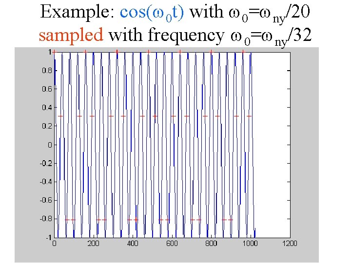
Example: cos(w 0 t) with w 0=wny/20 sampled with frequency w 0=wny/32

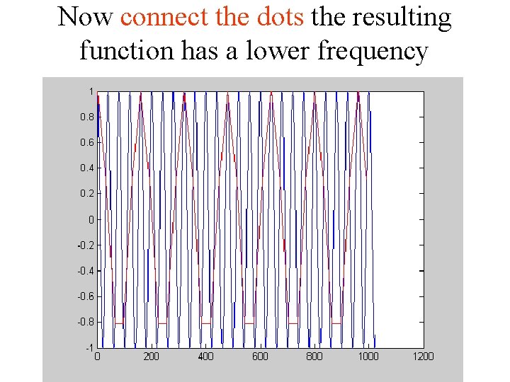
Now connect the dots the resulting function has a lower frequency

wn+N = wn let n=-m, then w-m = w. N-m

This is why the fourier coefficients of ‘negative frequencies’ are placed at the ‘high frequency’ end of the transform vector they “are” the high frequency coefficients

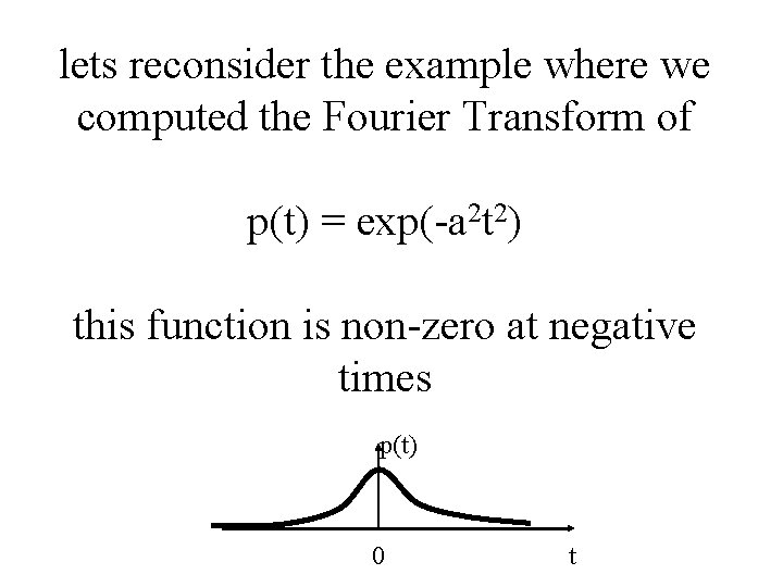
lets reconsider the example where we computed the Fourier Transform of p(t) = exp(-a 2 t 2) this function is non-zero at negative times p(t) 0 t

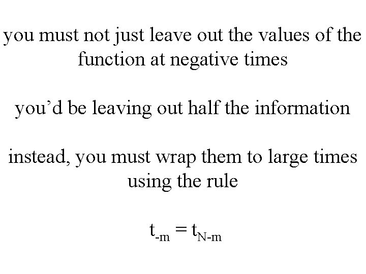
you must not just leave out the values of the function at negative times you’d be leaving out half the information instead, you must wrap them to large times using the rule t-m = t. N-m

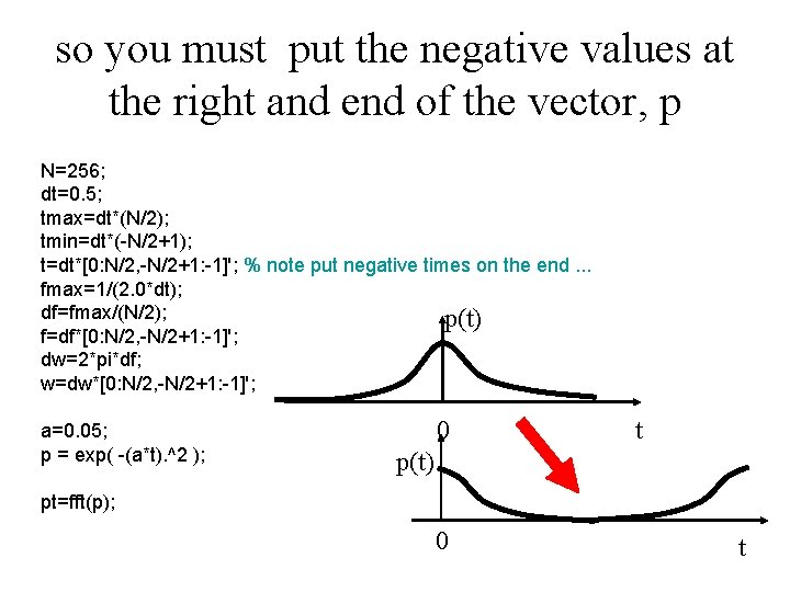
so you must put the negative values at the right and end of the vector, p N=256; dt=0. 5; tmax=dt*(N/2); tmin=dt*(-N/2+1); t=dt*[0: N/2, -N/2+1: -1]'; % note put negative times on the end. . . fmax=1/(2. 0*dt); df=fmax/(N/2); p(t) f=df*[0: N/2, -N/2+1: -1]'; dw=2*pi*df; w=dw*[0: N/2, -N/2+1: -1]'; a=0. 05; p = exp( -(a*t). ^2 ); 0 t p(t) pt=fft(p); 0 t

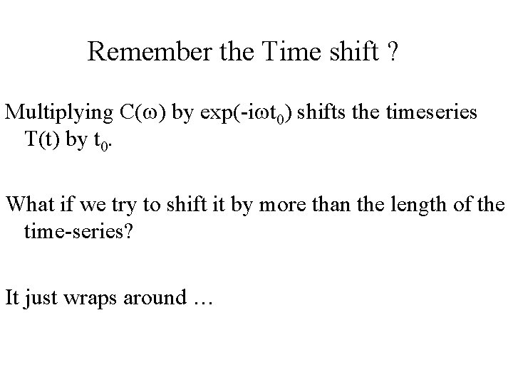
Remember the Time shift ? Multiplying C(w) by exp(-iwt 0) shifts the timeseries T(t) by t 0. What if we try to shift it by more than the length of the time-series? It just wraps around …

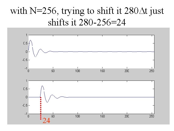
with N=256, trying to shift it 280 Dt just shifts it 280 -256=24 24