LECTURE 15 SECTIONS 7 3 7 5 Objectives

LECTURE 15 SECTIONS 7. 3 – 7. 5 Objectives: • More Large-Sample Confidence Intervals − Confidence Interval for π − Confidence Interval for µ 1 - µ 2 • Small sample intervals based on a Normal Population Distribution − t Distributions − One sample t confidence intervals − Confidence Interval for µ 1 - µ 2 − Paired sample confidence interval

LARGE SAMPLE CONFIDENCE INTERVAL FOR Π Recall that for large n, the sampling distribution of p is p ~ N(π , π (1−π )/n) approximately. This approximation is best when both nπ ≥ 5 and n(1−π ) ≥ 5. Notice that our textbook used 5 as a guide for large n in Chapter 5, but it is using 10 in Chapter 7. As I mentioned in Chapter 5, some books use 10 or 15 instead of 5. We will use 10 as a guide for large n in our class.

LARGE SAMPLE CONFIDENCE INTERVAL FOR Π Confidence intervals contain the population proportion π in C% of samples. For an SRS of size n drawn from a large population, and with sample proportion , p, calculated from the data, an approximate level C confidence interval for π is: C Use this method when the number of successes and the number of failures are both at least 10. m −Z* m Z* C is the area under the standard normal curve between −z* and z*.

EXAMPLE In n=48 trials in a particular laboratory, 16 resulted in ignition of a particular type of substrate by a lighted cigarette. Let π = the long-run proportion of all such trials that would result in ignition. Construct a 95% CI for π.

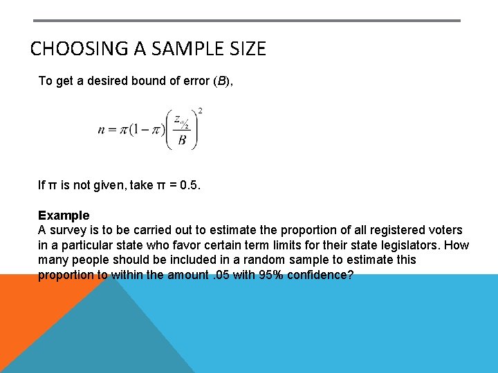
CHOOSING A SAMPLE SIZE To get a desired bound of error (B), If π is not given, take π = 0. 5. Example A survey is to be carried out to estimate the proportion of all registered voters in a particular state who favor certain term limits for their state legislators. How many people should be included in a random sample to estimate this proportion to within the amount. 05 with 95% confidence?

LARGE SAMPLE CONFIDENCE INTERVAL FOR Μ 1 - Μ 2 Now we have two different populations, processes, or treatments being compared. Consequently, we have two samples (each sample was randomly taken from a population). It is assumed that the observations in the first sample were obtained completely independently from those in the second sample. We have two independent SRSs (simple random samples) possibly coming from two distinct populations with (μ 1, σ1) and (μ 2, σ2) unknown. We use ( 1, s 1) and ( 2, s 2) to estimate (μ 1, σ1) and (μ 2, σ2) , respectively. To compare the means, both populations should be normally distributed. However, in practice, it is enough that the two distributions have similar shapes and that the sample data contain no strong outliers.

LARGE SAMPLE CONFIDENCE INTERVAL FOR Μ 1 Μ 2 Because we have two independent samples we use the difference between both sample averages ( 1− 2) to estimate (m 1 − m 2). Note: p C is the area between −z* and z*. p We find z* (the critical value) in Table I. p C The margin of error B is: B −z* B z*

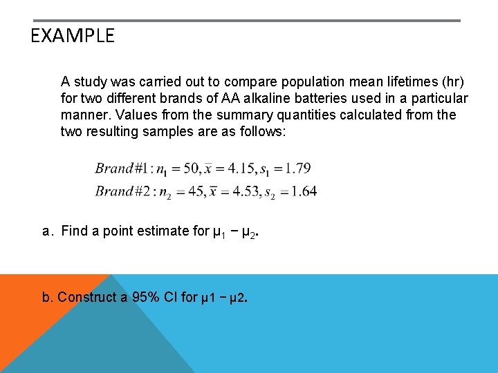
EXAMPLE A study was carried out to compare population mean lifetimes (hr) for two different brands of AA alkaline batteries used in a particular manner. Values from the summary quantities calculated from the two resulting samples are as follows: a. Find a point estimate for μ 1 − μ 2. b. Construct a 95% CI for μ 1 − μ 2.

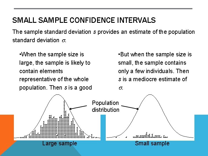
SMALL SAMPLE CONFIDENCE INTERVALS The sample standard deviation s provides an estimate of the population standard deviation s. • When the sample size is • But when the sample size is large, the sample is likely to small, the sample contains contain elements only a few individuals. Then representative of the whole s is a mediocre estimate of population. Then s is a good s. estimate of s. Population distribution Large sample Small sample

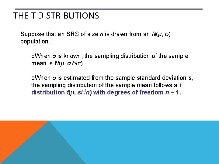
THE T DISTRIBUTIONS Suppose that an SRS of size n is drawn from an N(µ, σ) population. o. When σ is known, the sampling distribution of the sample mean is N(µ, σ /√n). o. When σ is estimated from the sample standard deviation s, the sampling distribution of the sample mean follows a t distribution t(µ, s/√n) with degrees of freedom n − 1.

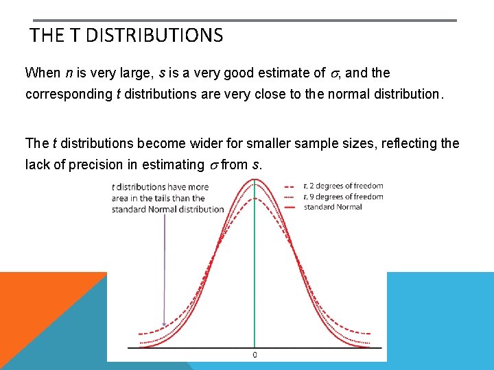
THE T DISTRIBUTIONS When n is very large, s is a very good estimate of s, and the corresponding t distributions are very close to the normal distribution. The t distributions become wider for smaller sample sizes, reflecting the lack of precision in estimating s from s.

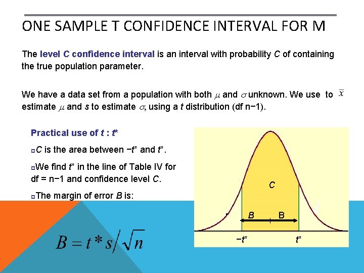
ONE SAMPLE T CONFIDENCE INTERVAL FOR Μ The level C confidence interval is an interval with probability C of containing the true population parameter. We have a data set from a population with both m and s unknown. We use to estimate m and s to estimate s, using a t distribution (df n− 1). Practical use of t : t* p C is the area between −t* and t*. We find t* in the line of Table IV for df = n− 1 and confidence level C. p p C The margin of error B is: B −t* B t*

SOME REMARKS Appendix Table IV gives a tabulation of such t critical values. Each row of the table corresponds to a different value of df, and each column gives critical values that capture a particular central area and the corresponding cumulative area. Notice that the validity of the above intervals requires that a population distribution be normal. You can check whether the data come from a normal population or not by drawing a normal quantile plot. If n is sufficiently large (n>30), the normality assumption is not necessary because of the CLT.

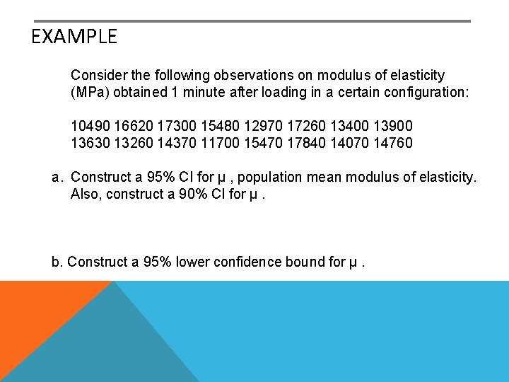
EXAMPLE Consider the following observations on modulus of elasticity (MPa) obtained 1 minute after loading in a certain configuration: 10490 16620 17300 15480 12970 17260 13400 13900 13630 13260 14370 11700 15470 17840 14070 14760 a. Construct a 95% CI for μ , population mean modulus of elasticity. Also, construct a 90% CI for μ. b. Construct a 95% lower confidence bound for μ.

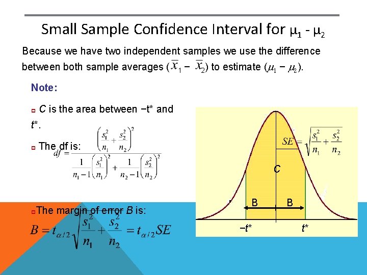
Small Sample Confidence Interval for µ 1 - µ 2 Because we have two independent samples we use the difference between both sample averages ( 1− 2) to estimate (m 1 − m 2). Note: p C is the area between −t* and t*. p The df is: C p The margin of error B is: B −t* B t*

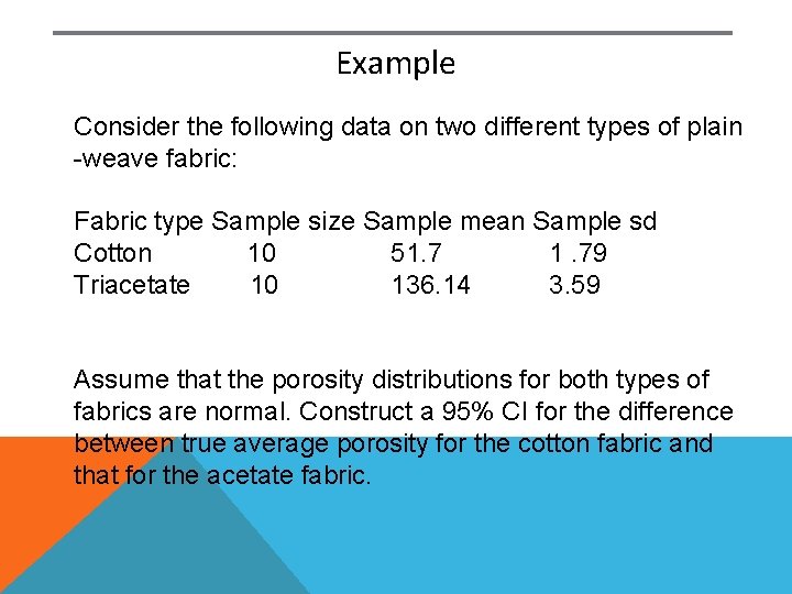
Example Consider the following data on two different types of plain -weave fabric: Fabric type Sample size Sample mean Sample sd Cotton 10 51. 79 Triacetate 10 136. 14 3. 59 Assume that the porosity distributions for both types of fabrics are normal. Construct a 95% CI for the difference between true average porosity for the cotton fabric and that for the acetate fabric.

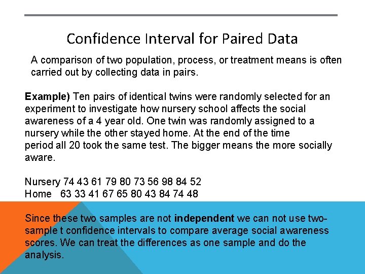
Confidence Interval for Paired Data A comparison of two population, process, or treatment means is often carried out by collecting data in pairs. Example) Ten pairs of identical twins were randomly selected for an experiment to investigate how nursery school affects the social awareness of a 4 year old. One twin was randomly assigned to a nursery while the other stayed home. At the end of the time period all 20 took the same test. The bigger means the more socially aware. Nursery 74 43 61 79 80 73 56 98 84 52 Home 63 33 41 67 65 80 43 84 74 48 Since these two samples are not independent we can not use twosample t confidence intervals to compare average social awareness scores. We can treat the differences as one sample and do the analysis.