Lecture 15 Review Session Todays topics FSM examples

Lecture 15: Review Session • Today’s topics: § FSM examples § Midterm review session § Midterm rules: This exam allows open book, open notes, open laptop, but no internet access. You may also not use the MARS simulator or other calculators and tools for numeric conversions. Use of calculators for other problems is ok. If necessary, make reasonable assumptions and clearly state them. The only clarifications you may ask for during the exam are definitions of terms. You'll receive partial credit if you show your steps and explain your line of thinking, so attempt every question even if you can't fully solve it. Complete your answers in the space provided (including the back-side of each page). Confirm that you have 15 questions on 7 pages, followed by a blank page. Turn in your answer sheets before 10: 35 am. The test is worth 100 points and you 1 have about 90 minutes, so allocate time accordingly.

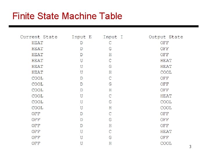
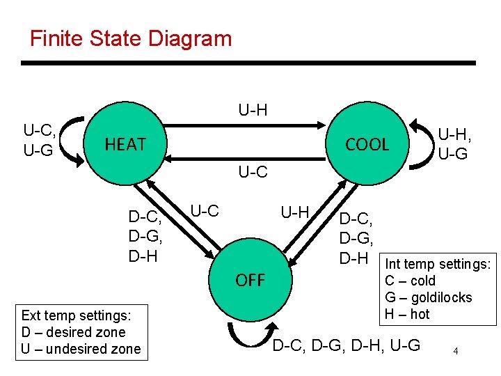
Example – Residential Thermostat • Two temp sensors: internal and external • If internal temp is within 1 degree of desired, don’t change setting • If internal temp is > 1 degree higher than desired, turn AC on; if internal temp is < 1 degree lower than desired, turn heater on • If external temp and desired temp are within 5 degrees, disregard the internal temp, and turn both AC and heater off 2

Finite State Machine Table 3

Finite State Diagram U-H U-C, U-G HEAT COOL U-C D-C, D-G, D-H U-C U-H OFF Ext temp settings: D – desired zone U – undesired zone U-H, U-G D-C, D-G, D-H Int temp settings: C – cold G – goldilocks H – hot D-C, D-G, D-H, U-G 4

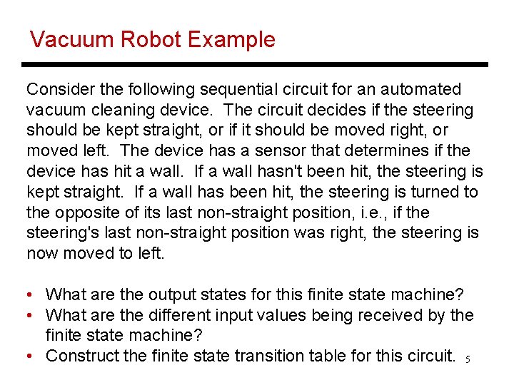
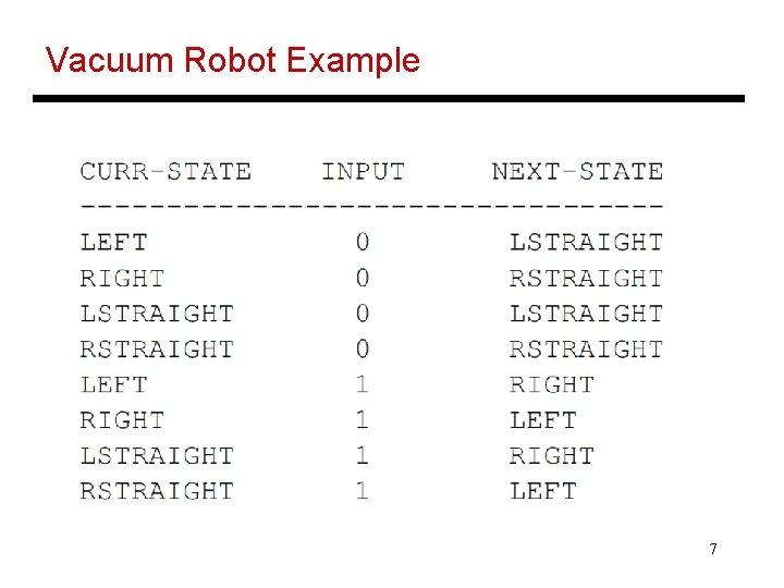
Vacuum Robot Example Consider the following sequential circuit for an automated vacuum cleaning device. The circuit decides if the steering should be kept straight, or if it should be moved right, or moved left. The device has a sensor that determines if the device has hit a wall. If a wall hasn't been hit, the steering is kept straight. If a wall has been hit, the steering is turned to the opposite of its last non-straight position, i. e. , if the steering's last non-straight position was right, the steering is now moved to left. • What are the output states for this finite state machine? • What are the different input values being received by the finite state machine? • Construct the finite state transition table for this circuit. 5

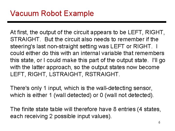
Vacuum Robot Example At first, the output of the circuit appears to be LEFT, RIGHT, STRAIGHT. But the circuit also needs to remember if the steering's last non-straight setting was LEFT or RIGHT. I could either do this with an internal variable that remembers this state, or I could make this part of the output state. I'll go with the latter approach, so the output states now become LEFT, RIGHT, LSTRAIGHT, RSTRAIGHT. There's only 1 input, which is the wall-detecting sensor, which is either 1 (wall detected) or 0 (wall not detected). The finite state table will therefore have 8 entries (4 states, each receiving 2 possible input values). 6

Vacuum Robot Example 7

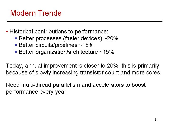
Modern Trends • Historical contributions to performance: § Better processes (faster devices) ~20% § Better circuits/pipelines ~15% § Better organization/architecture ~15% Today, annual improvement is closer to 20%; this is primarily because of slowly increasing transistor count and more cores. Need multi-thread parallelism and accelerators to boost performance every year. 8

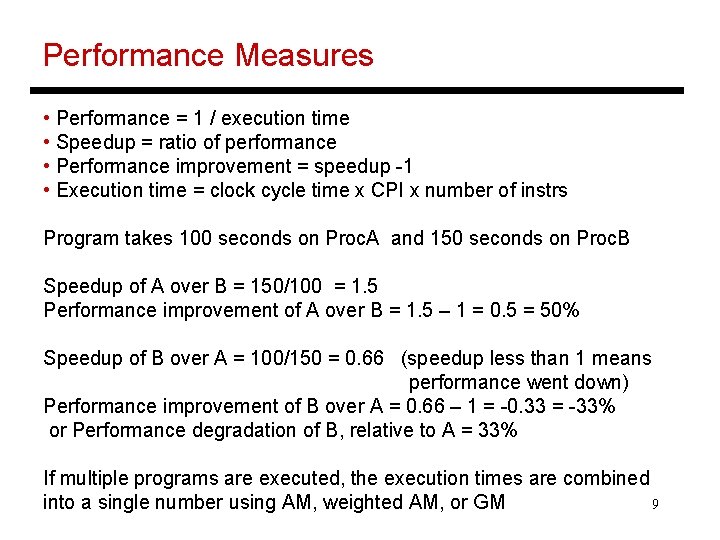
Performance Measures • Performance = 1 / execution time • Speedup = ratio of performance • Performance improvement = speedup -1 • Execution time = clock cycle time x CPI x number of instrs Program takes 100 seconds on Proc. A and 150 seconds on Proc. B Speedup of A over B = 150/100 = 1. 5 Performance improvement of A over B = 1. 5 – 1 = 0. 5 = 50% Speedup of B over A = 100/150 = 0. 66 (speedup less than 1 means performance went down) Performance improvement of B over A = 0. 66 – 1 = -0. 33 = -33% or Performance degradation of B, relative to A = 33% If multiple programs are executed, the execution times are combined into a single number using AM, weighted AM, or GM 9

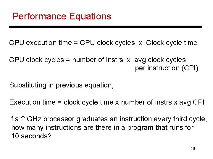
Performance Equations CPU execution time = CPU clock cycles x Clock cycle time CPU clock cycles = number of instrs x avg clock cycles per instruction (CPI) Substituting in previous equation, Execution time = clock cycle time x number of instrs x avg CPI If a 2 GHz processor graduates an instruction every third cycle, how many instructions are there in a program that runs for 10 seconds? 10

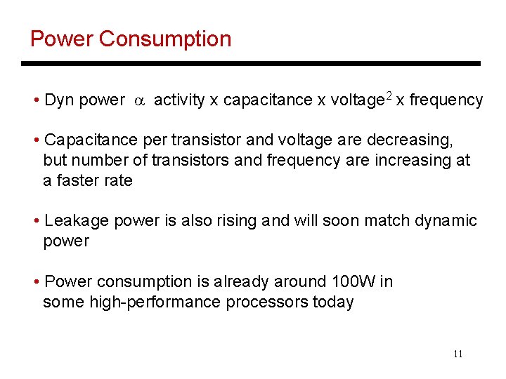
Power Consumption • Dyn power a activity x capacitance x voltage 2 x frequency • Capacitance per transistor and voltage are decreasing, but number of transistors and frequency are increasing at a faster rate • Leakage power is also rising and will soon match dynamic power • Power consumption is already around 100 W in some high-performance processors today 11

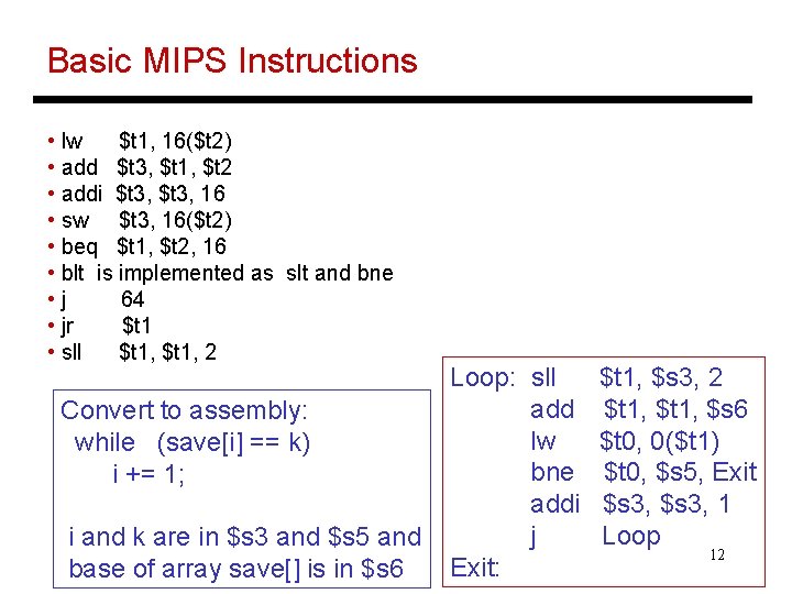
Basic MIPS Instructions • lw $t 1, 16($t 2) • add $t 3, $t 1, $t 2 • addi $t 3, 16 • sw $t 3, 16($t 2) • beq $t 1, $t 2, 16 • blt is implemented as slt and bne • j 64 • jr $t 1 • sll $t 1, 2 Convert to assembly: while (save[i] == k) i += 1; i and k are in $s 3 and $s 5 and base of array save[] is in $s 6 Loop: sll add lw bne addi j Exit: $t 1, $s 3, 2 $t 1, $s 6 $t 0, 0($t 1) $t 0, $s 5, Exit $s 3, 1 Loop 12

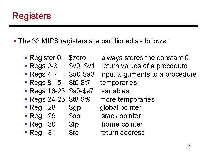
Registers • The 32 MIPS registers are partitioned as follows: § Register 0 : $zero § Regs 2 -3 : $v 0, $v 1 § Regs 4 -7 : $a 0 -$a 3 § Regs 8 -15 : $t 0 -$t 7 § Regs 16 -23: $s 0 -$s 7 § Regs 24 -25: $t 8 -$t 9 § Reg 28 : $gp § Reg 29 : $sp § Reg 30 : $fp § Reg 31 : $ra always stores the constant 0 return values of a procedure input arguments to a procedure temporaries variables more temporaries global pointer stack pointer frame pointer return address 13

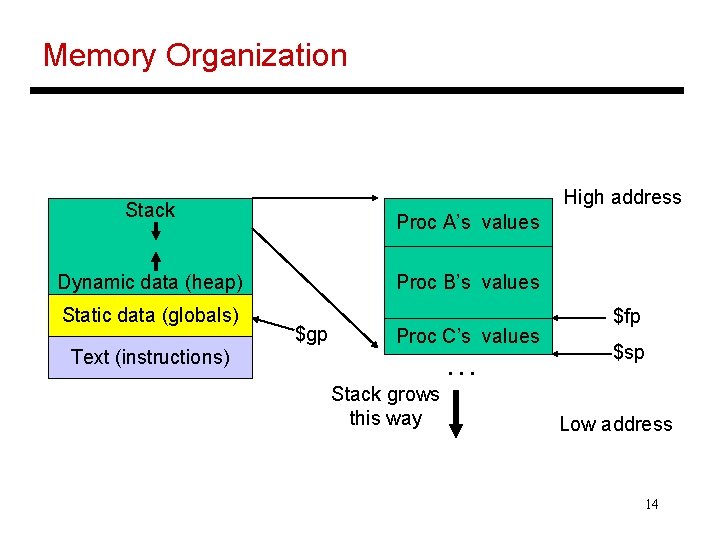
Memory Organization High address Stack Proc A’s values Proc B’s values Dynamic data (heap) Static data (globals) Text (instructions) $gp Proc C’s values … Stack grows this way $fp $sp Low address 14

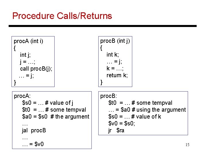
Procedure Calls/Returns proc. A (int i) { int j; j = …; call proc. B(j); … = j; } proc. B (int j) { int k; … = j; k = …; return k; } proc. A: $s 0 = … # value of j $t 0 = … # some tempval $a 0 = $s 0 # the argument … jal proc. B … … = $v 0 proc. B: $t 0 = … # some tempval … = $a 0 # using the argument $s 0 = … # value of k $v 0 = $s 0; jr $ra 15

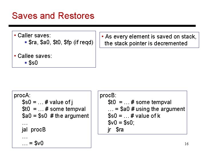
Saves and Restores • Caller saves: § $ra, $a 0, $t 0, $fp (if reqd) • As every element is saved on stack, the stack pointer is decremented • Callee saves: § $s 0 proc. A: $s 0 = … # value of j $t 0 = … # some tempval $a 0 = $s 0 # the argument … jal proc. B … … = $v 0 proc. B: $t 0 = … # some tempval … = $a 0 # using the argument $s 0 = … # value of k $v 0 = $s 0; jr $ra 16

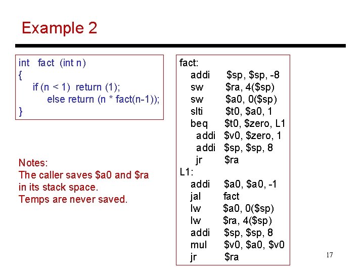
Example 2 int fact (int n) { if (n < 1) return (1); else return (n * fact(n-1)); } Notes: The caller saves $a 0 and $ra in its stack space. Temps are never saved. fact: addi sw sw slti beq addi jr L 1: addi jal lw lw addi mul jr $sp, -8 $ra, 4($sp) $a 0, 0($sp) $t 0, $a 0, 1 $t 0, $zero, L 1 $v 0, $zero, 1 $sp, 8 $ra $a 0, -1 fact $a 0, 0($sp) $ra, 4($sp) $sp, 8 $v 0, $a 0, $v 0 $ra 17

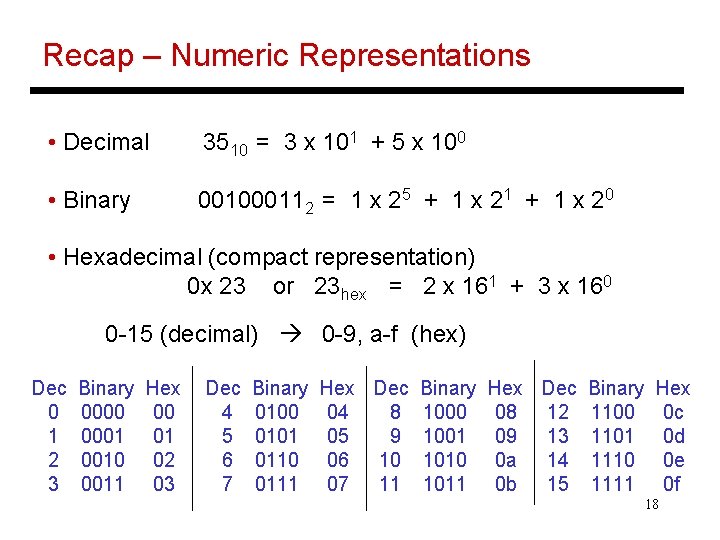
Recap – Numeric Representations • Decimal 3510 = 3 x 101 + 5 x 100 • Binary 001000112 = 1 x 25 + 1 x 21 + 1 x 20 • Hexadecimal (compact representation) 0 x 23 or 23 hex = 2 x 161 + 3 x 160 0 -15 (decimal) 0 -9, a-f (hex) Dec 0 1 2 3 Binary 0000 0001 0010 0011 Hex 00 01 02 03 Dec 4 5 6 7 Binary 0100 0101 0110 0111 Hex Dec Binary 04 8 1000 05 9 1001 06 10 1010 07 11 1011 Hex Dec Binary 08 12 1100 09 13 1101 0 a 14 1110 0 b 15 1111 Hex 0 c 0 d 0 e 0 f 18

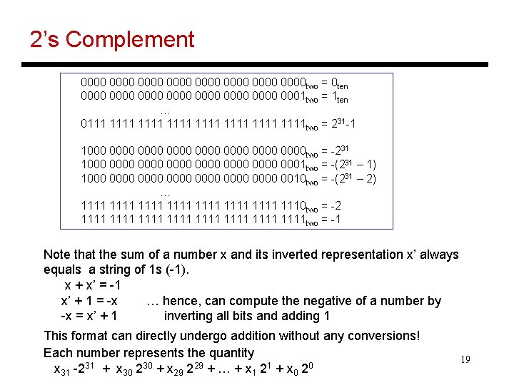
2’s Complement 0000 0000 two = 0 ten 0000 0000 0001 two = 1 ten … 0111 1111 1111 two = 231 -1 1000 0000 0000 two = -231 1000 0000 0000 0001 two = -(231 – 1) 1000 0000 0000 0010 two = -(231 – 2) … 1111 1111 1110 two = -2 1111 1111 two = -1 Note that the sum of a number x and its inverted representation x’ always equals a string of 1 s (-1). x + x’ = -1 x’ + 1 = -x … hence, can compute the negative of a number by -x = x’ + 1 inverting all bits and adding 1 This format can directly undergo addition without any conversions! Each number represents the quantity x 31 -231 + x 30 230 + x 29 229 + … + x 1 21 + x 0 20 19

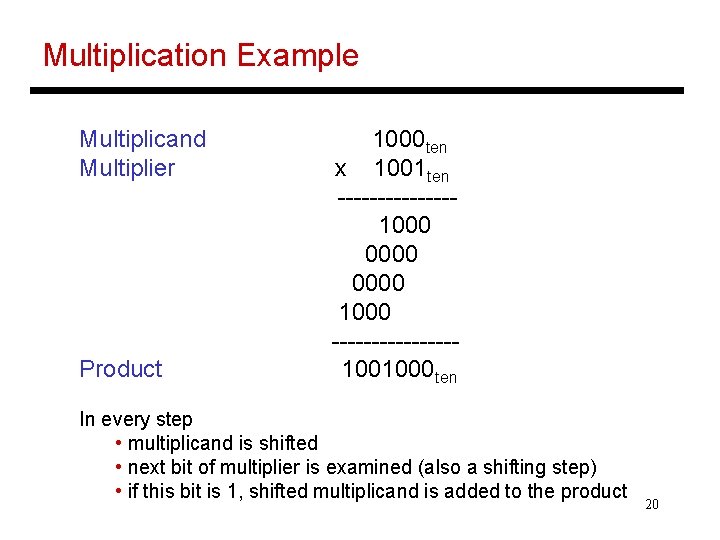
Multiplication Example Multiplicand Multiplier Product 1000 ten x 1001 ten -------1000 0000 1000 --------1001000 ten In every step • multiplicand is shifted • next bit of multiplier is examined (also a shifting step) • if this bit is 1, shifted multiplicand is added to the product 20

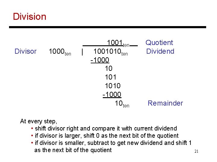
Division Divisor 1000 ten | 1001 ten 1001010 ten -1000 10 1010 -1000 10 ten Quotient Dividend Remainder At every step, • shift divisor right and compare it with current dividend • if divisor is larger, shift 0 as the next bit of the quotient • if divisor is smaller, subtract to get new dividend and shift 1 as the next bit of the quotient 21

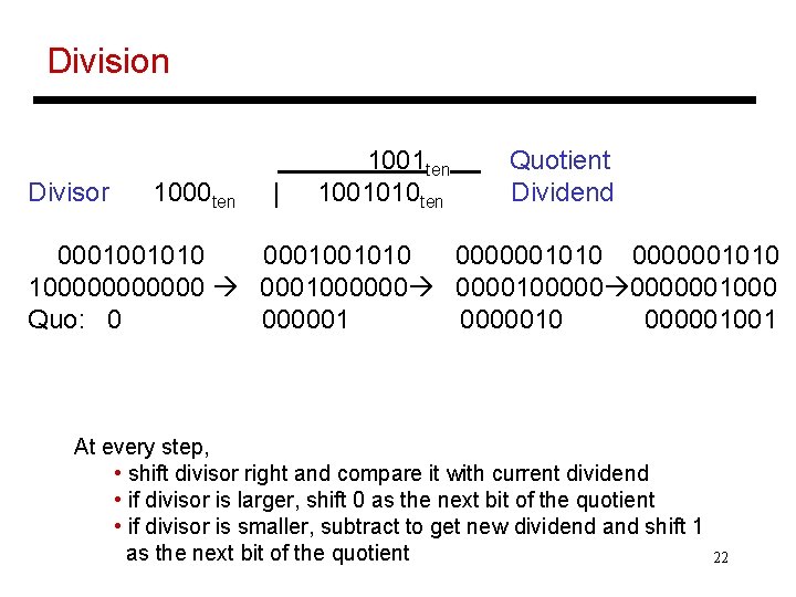
Division Divisor 1000 ten | 1001 ten 1001010 ten Quotient Dividend 0001001010 0000001010 1000000 000100000010000001000 Quo: 0 000001001 At every step, • shift divisor right and compare it with current dividend • if divisor is larger, shift 0 as the next bit of the quotient • if divisor is smaller, subtract to get new dividend and shift 1 as the next bit of the quotient 22

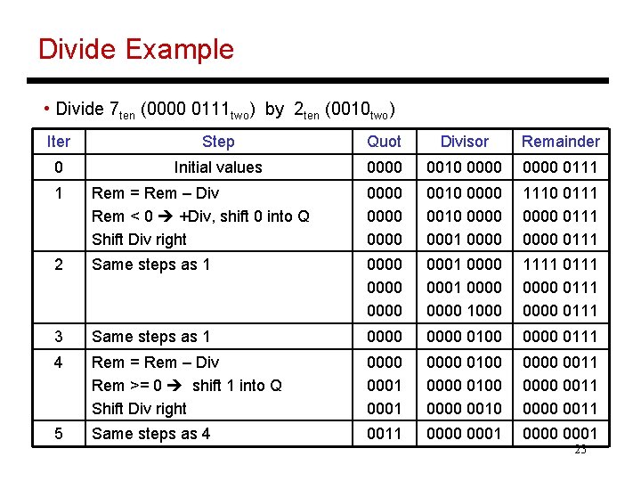
Divide Example • Divide 7 ten (0000 0111 two) by 2 ten (0010 two) Iter Step Quot Divisor Remainder 0 Initial values 0000 0010 0000 0111 1 Rem = Rem – Div Rem < 0 +Div, shift 0 into Q Shift Div right 0000 0010 0000 0001 0000 1110 0111 0000 0111 2 Same steps as 1 0000 0001 0000 1000 1111 0000 0111 3 Same steps as 1 0000 0100 0000 0111 4 Rem = Rem – Div Rem >= 0 shift 1 into Q Shift Div right 0000 0001 0000 0100 0000 0010 0000 0011 5 Same steps as 4 0011 0000 0001 23

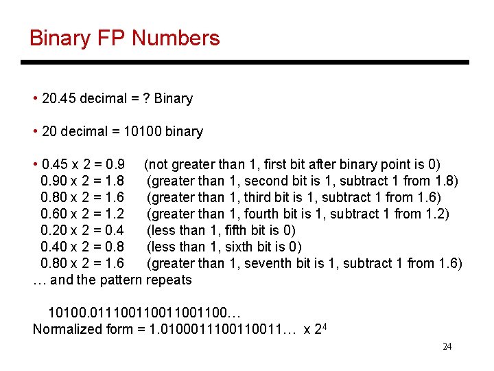
Binary FP Numbers • 20. 45 decimal = ? Binary • 20 decimal = 10100 binary • 0. 45 x 2 = 0. 9 (not greater than 1, first bit after binary point is 0) 0. 90 x 2 = 1. 8 (greater than 1, second bit is 1, subtract 1 from 1. 8) 0. 80 x 2 = 1. 6 (greater than 1, third bit is 1, subtract 1 from 1. 6) 0. 60 x 2 = 1. 2 (greater than 1, fourth bit is 1, subtract 1 from 1. 2) 0. 20 x 2 = 0. 4 (less than 1, fifth bit is 0) 0. 40 x 2 = 0. 8 (less than 1, sixth bit is 0) 0. 80 x 2 = 1. 6 (greater than 1, seventh bit is 1, subtract 1 from 1. 6) … and the pattern repeats 10100. 0111001100… Normalized form = 1. 010001110011… x 24 24

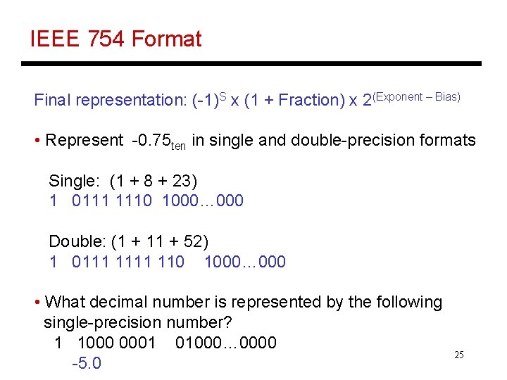
IEEE 754 Format Final representation: (-1)S x (1 + Fraction) x 2(Exponent – Bias) • Represent -0. 75 ten in single and double-precision formats Single: (1 + 8 + 23) 1 0111 1110 1000… 000 Double: (1 + 11 + 52) 1 0111 110 1000… 000 • What decimal number is represented by the following single-precision number? 1 1000 0001 01000… 0000 -5. 0 25

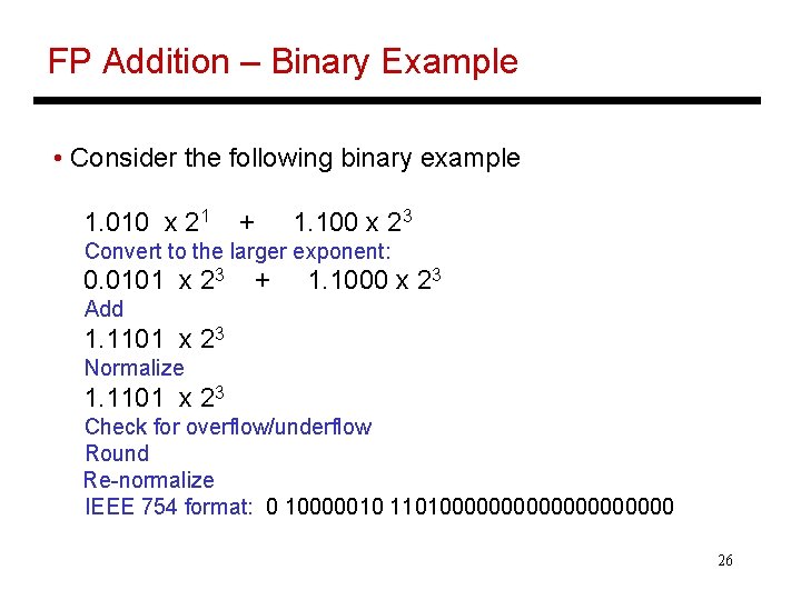
FP Addition – Binary Example • Consider the following binary example 1. 010 x 21 + 1. 100 x 23 Convert to the larger exponent: 0. 0101 x 23 + 1. 1000 x 23 Add 1. 1101 x 23 Normalize 1. 1101 x 23 Check for overflow/underflow Round Re-normalize IEEE 754 format: 0 10000010 11010000000000 26

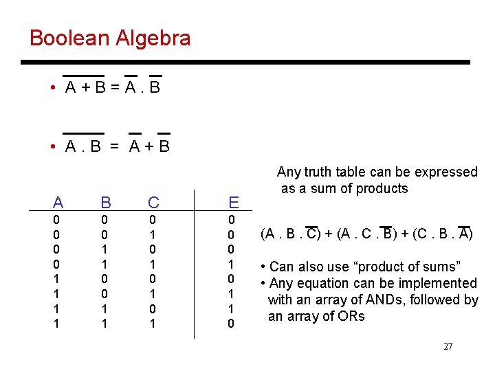
Boolean Algebra • A+B=A. B • A. B = A+B A B C E 0 0 1 1 0 1 0 1 0 0 0 1 1 0 Any truth table can be expressed as a sum of products (A. B. C) + (A. C. B) + (C. B. A) • Can also use “product of sums” • Any equation can be implemented with an array of ANDs, followed by an array of ORs 27

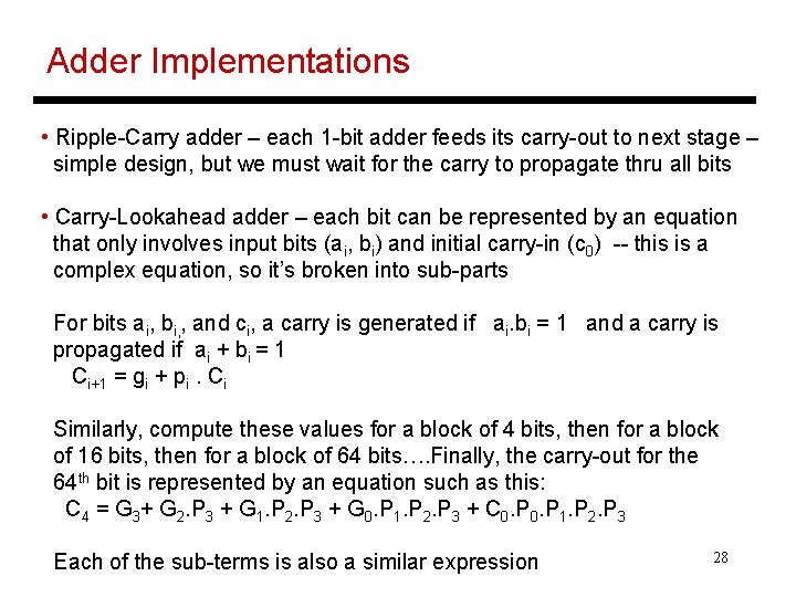
Adder Implementations • Ripple-Carry adder – each 1 -bit adder feeds its carry-out to next stage – simple design, but we must wait for the carry to propagate thru all bits • Carry-Lookahead adder – each bit can be represented by an equation that only involves input bits (ai, bi) and initial carry-in (c 0) -- this is a complex equation, so it’s broken into sub-parts For bits ai, bi, , and ci, a carry is generated if ai. bi = 1 and a carry is propagated if ai + bi = 1 Ci+1 = gi + pi. Ci Similarly, compute these values for a block of 4 bits, then for a block of 16 bits, then for a block of 64 bits…. Finally, the carry-out for the 64 th bit is represented by an equation such as this: C 4 = G 3+ G 2. P 3 + G 1. P 2. P 3 + G 0. P 1. P 2. P 3 + C 0. P 1. P 2. P 3 Each of the sub-terms is also a similar expression 28

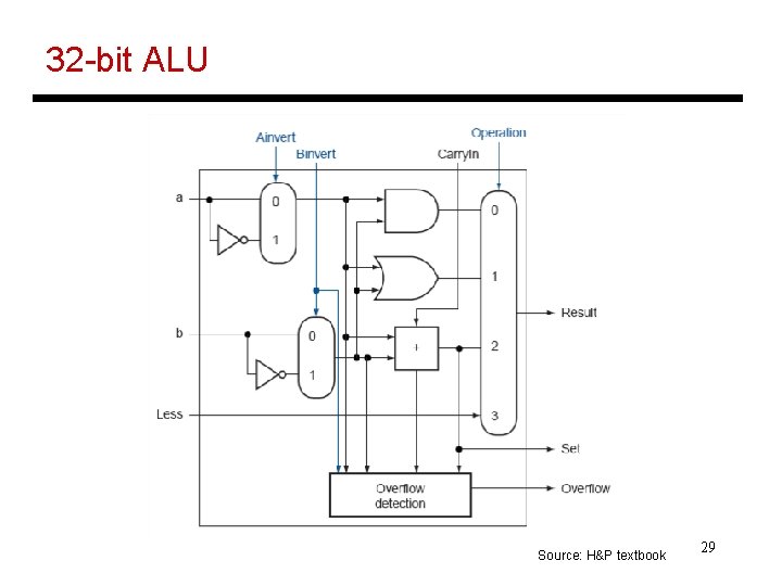
32 -bit ALU Source: H&P textbook 29

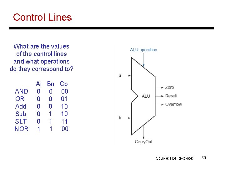
Control Lines What are the values of the control lines and what operations do they correspond to? AND OR Add Sub SLT NOR Ai Bn Op 0 0 0 01 0 0 1 10 0 1 11 1 1 00 Source: H&P textbook 30