Lecture 15 Persistence Database Management Systems 1 Data

Lecture 15 Persistence Database Management Systems 1

Data Storage and Persistence • Data in RAM: • Data saved in virtual memory is gone, when a process ends • The memory space is free to be used by other processes currently being executed. • Data Storage: • Data in storage remains unchanged beyond the end of the process lifecycle • RTE provides services to processes to support data storage • Examples: HDD, SD-Cards, CD, DVD, Blu-Ray, etc…

Persistence: Persistent Data Storage • Persistent Data: • Data that is stored in some storage mechanism • In addition, it can be shared amongst multiple executing processes • Examples: • File System – in every data storage location • Databases – Relational Databases, and Document Oriented Databases • In other words: SQL and No. SQL databases • We will introduce an introduction to SQL databases

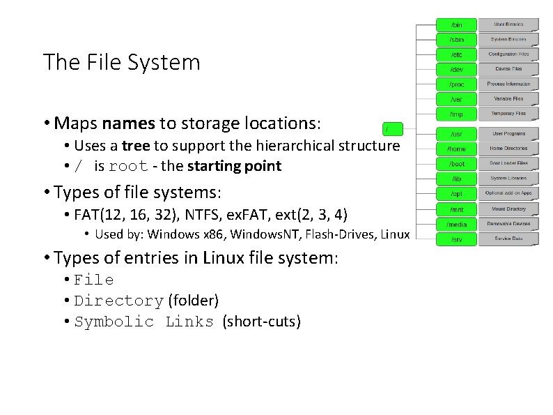
The File System • Maps names to storage locations: • Uses a tree to support the hierarchical structure • / is root - the starting point • Types of file systems: • FAT(12, 16, 32), NTFS, ex. FAT, ext(2, 3, 4) • Used by: Windows x 86, Windows. NT, Flash-Drives, Linux • Types of entries in Linux file system: • File • Directory (folder) • Symbolic Links (short-cuts)

File System Services • Access through streams: • Stream interface to read and write a file as a stream of bytes. • FS allows to seek within the file, read its content and write new content. • Allocation of space / automatic increase storage space (in writes). • Locking files: • Allows multiple processes to synchronize access on shared files. • One can lock a whole file or just a segment of bytes within the content of a file. 5

File Systems • FS provides abstract interface of system calls (open, read, write, seek etc) • implemented by specific drivers which know how to interact with specific hardware devices. • Distributed FS: • process can request access to files stored on a remote machine: • Local FS in RTE passes the system calls (open, read, etc. ) to FS-server on server • Distributed file systems (for example, NFS and SAMBA) have complex locking mechanisms. 6

Database Management System (DBMS) 1. Another way to store persistent data. 2. DBMS is present as a service. 3. Processes connect through inter-process communication protocol (over TCP). 4. DBMS manages storage, often by accessing FS on its side. 7

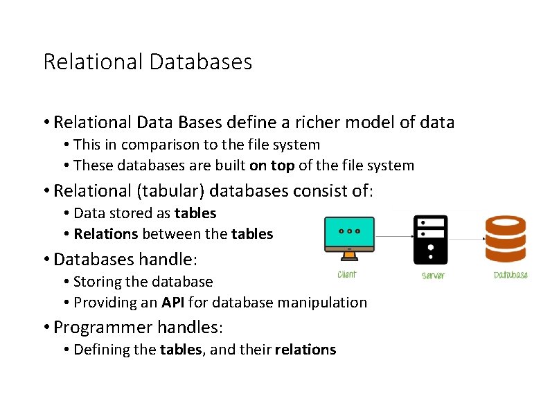
Relational Databases • Relational Data Bases define a richer model of data • This in comparison to the file system • These databases are built on top of the file system • Relational (tabular) databases consist of: • Data stored as tables • Relations between the tables • Databases handle: • Storing the database • Providing an API for database manipulation • Programmer handles: • Defining the tables, and their relations

File systems vs. DBMS - differences • DBMS can define rich data models. • FS is very simple: a stream of bytes. • DBMS manages encoding / decoding. • Programmers define the specific data model they are interested in using. • Databases provide an interface for data storage and manipulation • The programmer uses the interface to execute its queries • API is access by using the database management system (object) 9

File systems vs. DBMS • Efficient concurrency • DBMSs are built to support thousands of concurrent users. • Ensure data is kept consistent. • Optimized queries. Parallel-safe. • Not directly visible to user: • File and Access methods. • Buffer management. • Disk space management. 10

DBMS Services • Security management: • Verify that users are authorized to access data. • Specific rights can be granted for each part of the data and each group of users. • Session and Transaction management: • Users execute data transactions. • Transaction = complex data operation: • read and modify many different objects • Viewed from the outside as a single atomic operation - completely succeeds or not performed. • If completed successfully, transactions must be committed to the storage. 11

Transaction • A transaction is usually issued to the DB in a language like SQL, using a pattern like: • Begin transaction. • Execute data manipulations and queries. • If no errors occur then commit transaction. • If errors occur rollback the transaction. 12

Transaction • Transaction safety. • Modifications performed on snapshot in memory. • Isolation: intermediate modifications not committed are not visible to other threads. • Transaction committed: modifications are merged to persistent storage • If transaction is rollbacked: modifications are deleted and the storage is not modified. 13

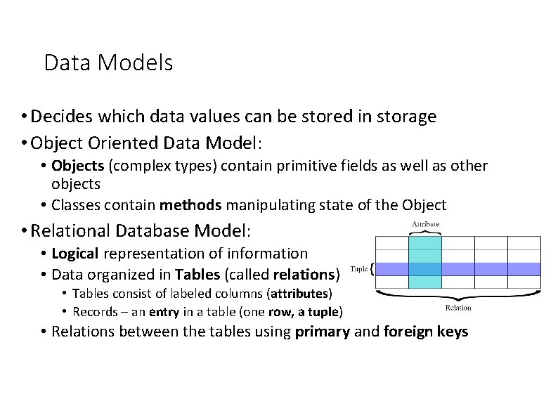
Data Models • Decides which data values can be stored in storage • Object Oriented Data Model: • Objects (complex types) contain primitive fields as well as other objects • Classes contain methods manipulating state of the Object • Relational Database Model: • Logical representation of information • Data organized in Tables (called relations) • Tables consist of labeled columns (attributes) • Records – an entry in a table (one row, a tuple) • Relations between the tables using primary and foreign keys

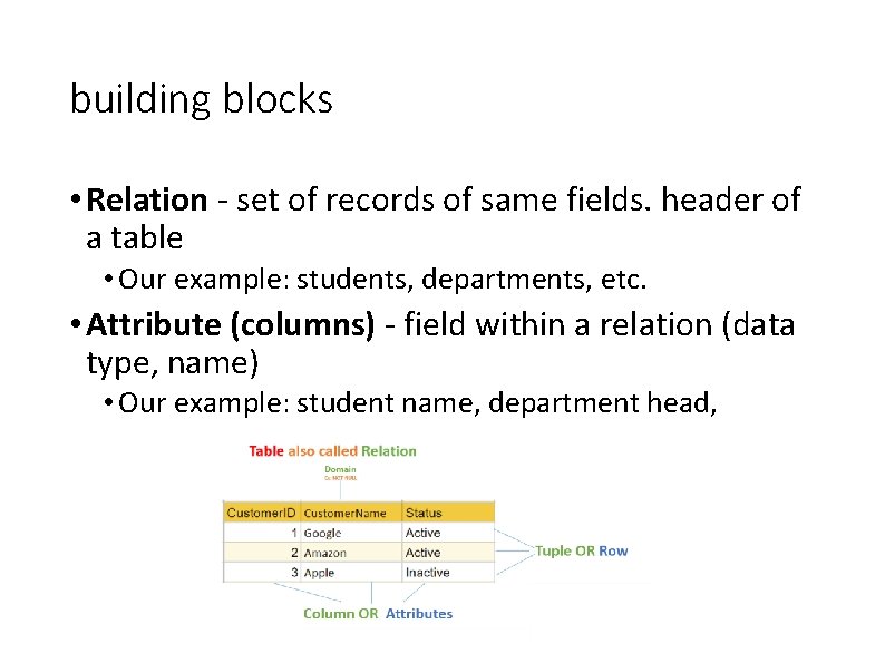
building blocks • Relation - set of records of same fields. header of a table • Our example: students, departments, etc. • Attribute (columns) - field within a relation (data type, name) • Our example: student name, department head, 15

building blocks • Domain - restriction of data types • our example: student ID is 9 digits 0 -9 each. • Records - (or tuple), single row within a relation. • Integrity constraints - constraint on attribute with regard to all records • our example: Student ID is unique. 16

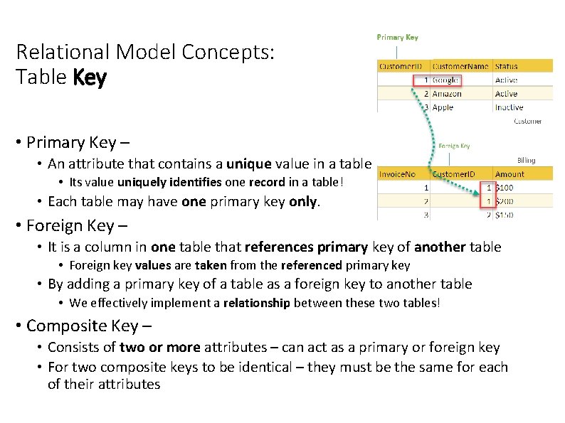
Relational Model Concepts: Table Key • Primary Key – • An attribute that contains a unique value in a table • Its value uniquely identifies one record in a table! • Each table may have one primary key only. • Foreign Key – • It is a column in one table that references primary key of another table • Foreign key values are taken from the referenced primary key • By adding a primary key of a table as a foreign key to another table • We effectively implement a relationship between these two tables! • Composite Key – • Consists of two or more attributes – can act as a primary or foreign key • For two composite keys to be identical – they must be the same for each of their attributes

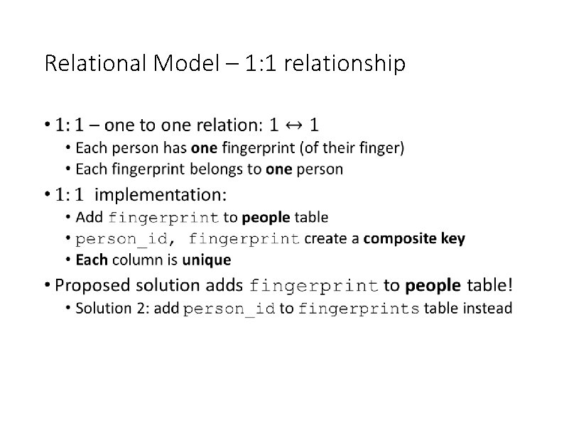
Relational Model – 1: 1 relationship •

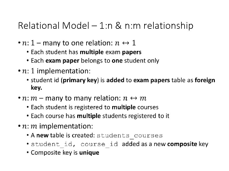
Relational Model – 1: n & n: m relationship •

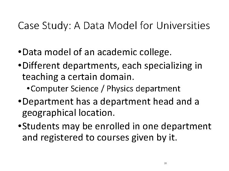
Case Study: A Data Model for Universities • Data model of an academic college. • Different departments, each specializing in teaching a certain domain. • Computer Science / Physics department • Department has a department head and a geographical location. • Students may be enrolled in one department and registered to courses given by it. 20

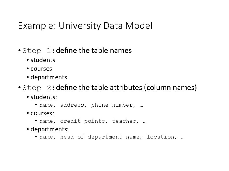
Example: University Data Model • Step 1: define the table names • students • courses • departments • Step 2: define the table attributes (column names) • students: • name, address, phone number, … • courses: • name, credit points, teacher, … • departments: • name, head of department name, location, …

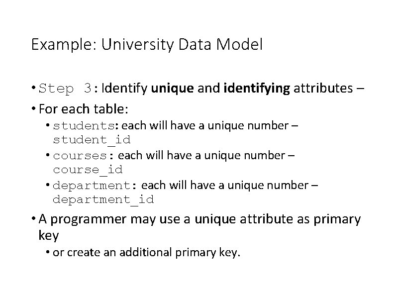
Example: University Data Model • Step 3: Identify unique and identifying attributes – • For each table: • students: each will have a unique number – student_id • courses: each will have a unique number – course_id • department: each will have a unique number – department_id • A programmer may use a unique attribute as primary key • or create an additional primary key.

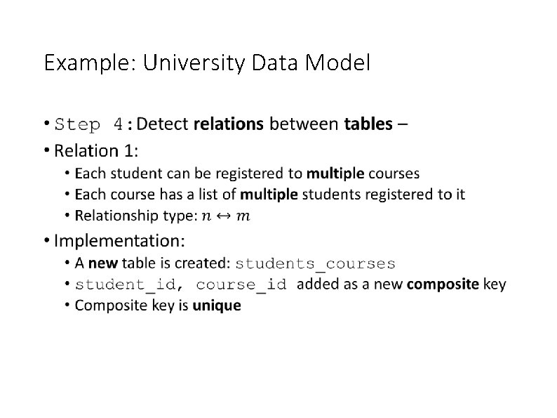
Example: University Data Model •

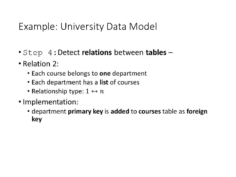
Example: University Data Model •

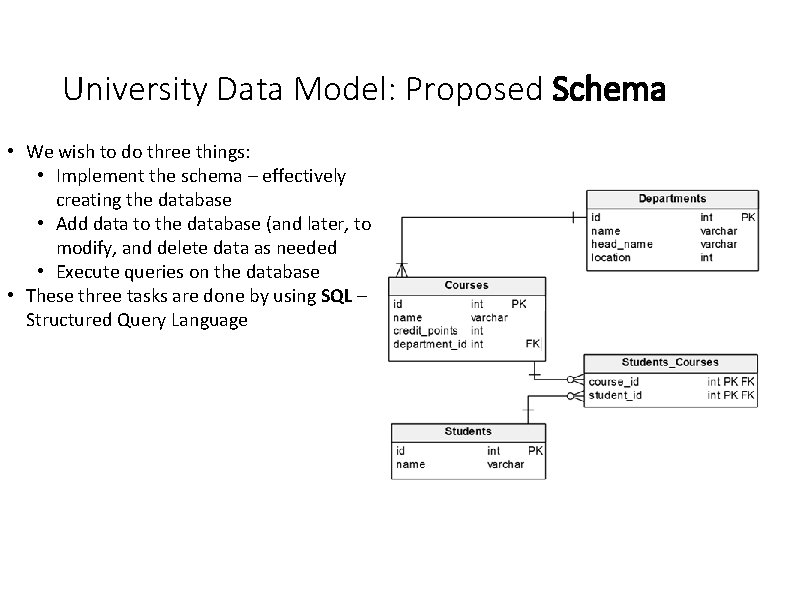
University Data Model: Proposed Schema • We wish to do three things: • Implement the schema – effectively creating the database • Add data to the database (and later, to modify, and delete data as needed • Execute queries on the database • These three tasks are done by using SQL – Structured Query Language

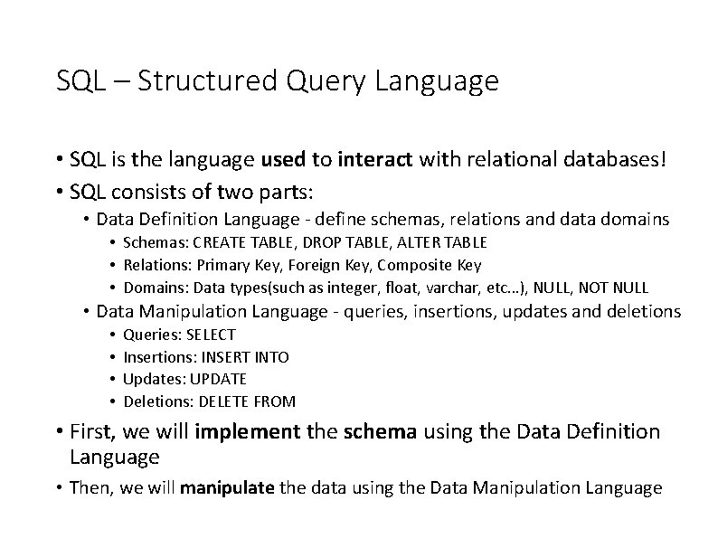
SQL – Structured Query Language • SQL is the language used to interact with relational databases! • SQL consists of two parts: • Data Definition Language - define schemas, relations and data domains • Schemas: CREATE TABLE, DROP TABLE, ALTER TABLE • Relations: Primary Key, Foreign Key, Composite Key • Domains: Data types(such as integer, float, varchar, etc…), NULL, NOT NULL • Data Manipulation Language - queries, insertions, updates and deletions • • Queries: SELECT Insertions: INSERT INTO Updates: UPDATE Deletions: DELETE FROM • First, we will implement the schema using the Data Definition Language • Then, we will manipulate the data using the Data Manipulation Language

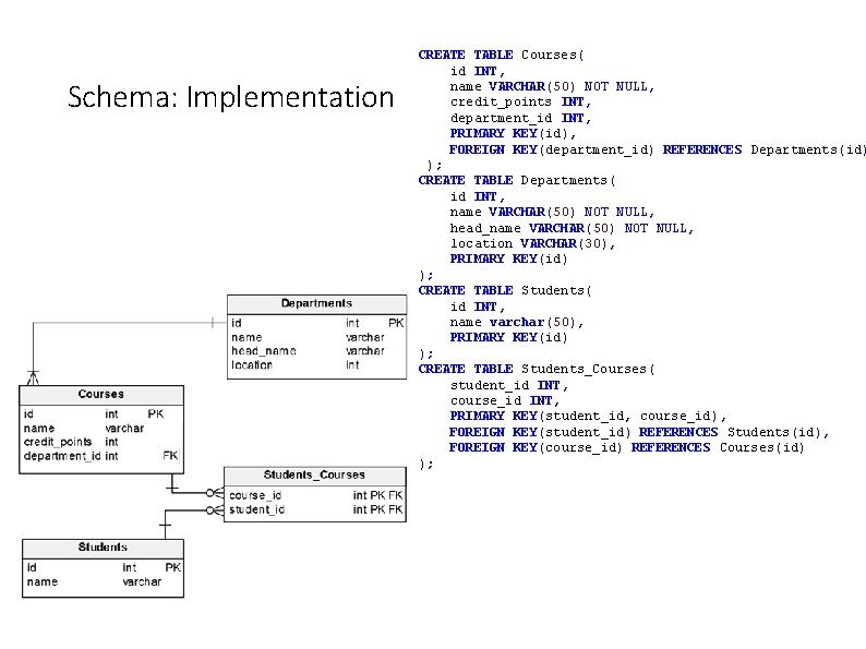
Schema: Implementation CREATE TABLE Courses( id INT, name VARCHAR(50) NOT NULL, credit_points INT, department_id INT, PRIMARY KEY(id), FOREIGN KEY(department_id) REFERENCES Departments(id) ); CREATE TABLE Departments( id INT, name VARCHAR(50) NOT NULL, head_name VARCHAR(50) NOT NULL, location VARCHAR(30), PRIMARY KEY(id) ); CREATE TABLE Students( id INT, name varchar(50), PRIMARY KEY(id) ); CREATE TABLE Students_Courses( student_id INT, course_id INT, PRIMARY KEY(student_id, course_id), FOREIGN KEY(student_id) REFERENCES Students(id), FOREIGN KEY(course_id) REFERENCES Courses(id) );

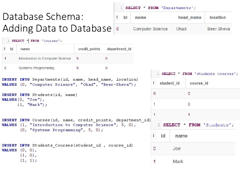
Database Schema: Adding Data to Database INSERT INTO Departments(id, name, head_name, location) VALUES (0, "Computer Science", "Ohad", "Beer-Sheva"); INSERT INTO Students(id, name) VALUES(0, "Joe"), (1, "Mark"); INSERT INTO Courses(id, name, credit_points, department_id) VALUES (1, "Introduction to Computer Science", 5, 0), (0, "Systems Programming", 5, 0); INSERT INTO Students_Courses(student_id , course_id) VALUES (0, 0), (1, 1);

Relational Algebra: executing querries • Selection - select specific rows from a relation. • Projection - projects specific columns • Set operations - union, intersection, crossproduct, set-difference • on relations that have the same structure (same attributes) • Join - cross product followed by selection and projection. • Renaming operation - change name of columns. 29

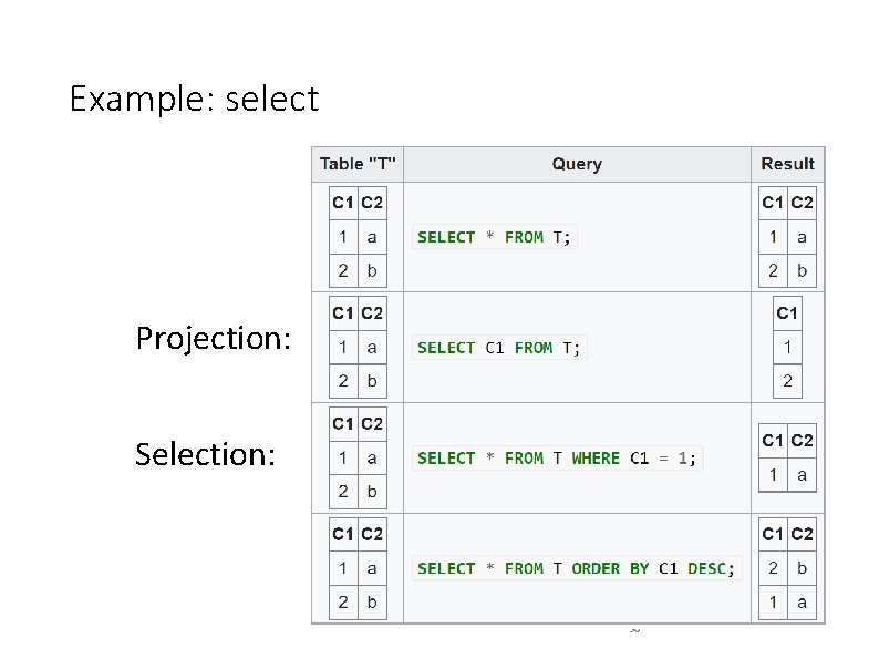
Example: select Projection: Selection: 30

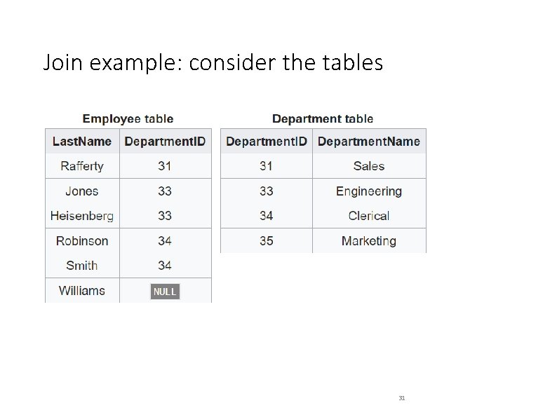
Join example: consider the tables 31

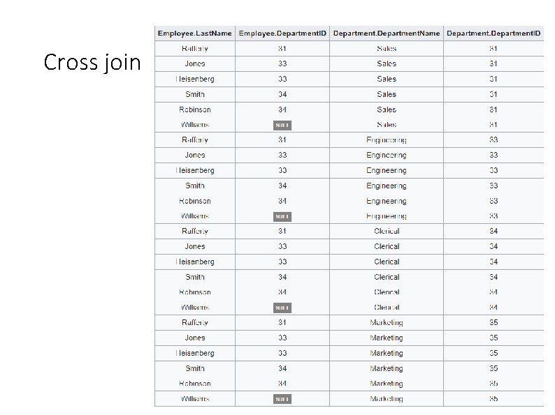
Cross join 32

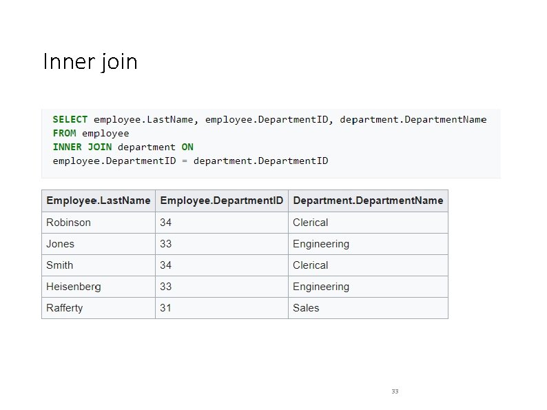
Inner join 33

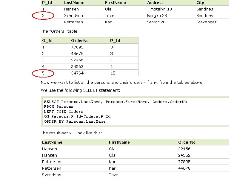
34

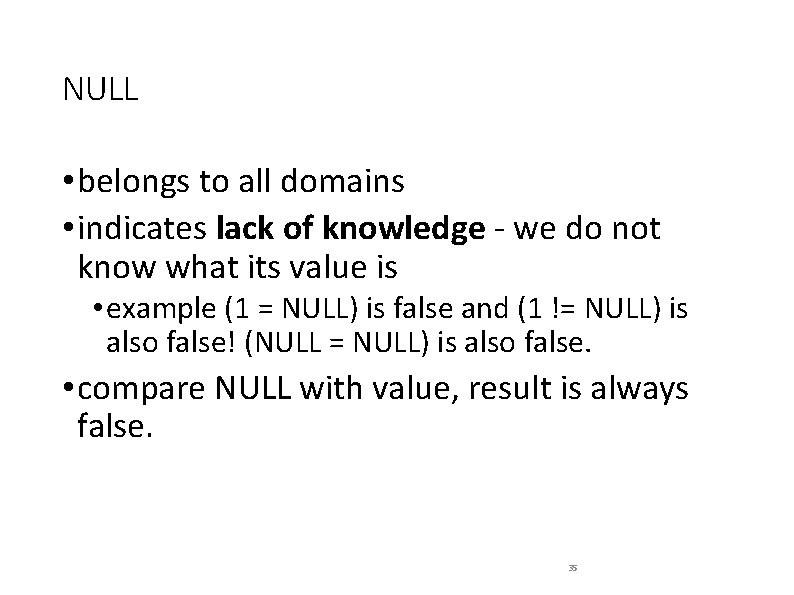
NULL • belongs to all domains • indicates lack of knowledge - we do not know what its value is • example (1 = NULL) is false and (1 != NULL) is also false! (NULL = NULL) is also false. • compare NULL with value, result is always false. 35

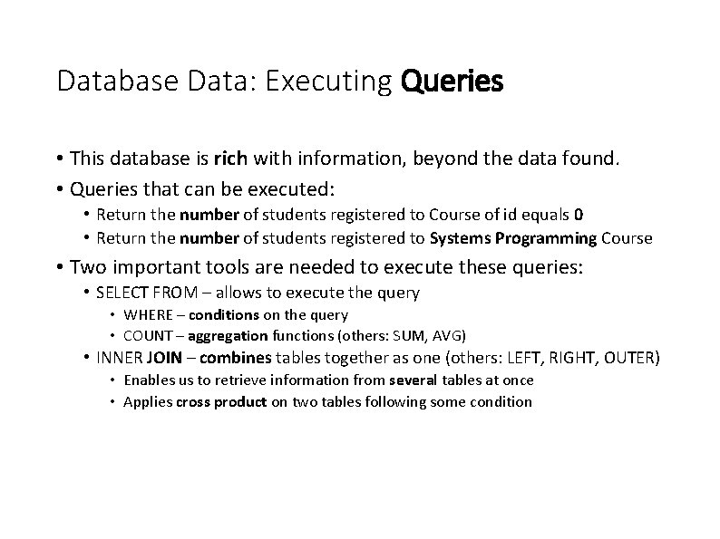
Database Data: Executing Queries • This database is rich with information, beyond the data found. • Queries that can be executed: • Return the number of students registered to Course of id equals 0 • Return the number of students registered to Systems Programming Course • Two important tools are needed to execute these queries: • SELECT FROM – allows to execute the query • WHERE – conditions on the query • COUNT – aggregation functions (others: SUM, AVG) • INNER JOIN – combines tables together as one (others: LEFT, RIGHT, OUTER) • Enables us to retrieve information from several tables at once • Applies cross product on two tables following some condition

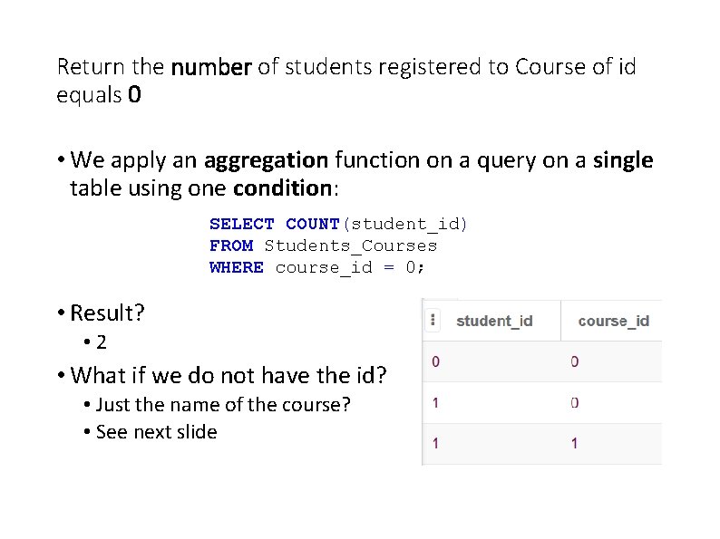
Return the number of students registered to Course of id equals 0 • We apply an aggregation function on a query on a single table using one condition: SELECT COUNT(student_id) FROM Students_Courses WHERE course_id = 0; • Result? • 2 • What if we do not have the id? • Just the name of the course? • See next slide

Return the number of students registered to Systems Programming Course • In this case we don’t know the id, but we have its name • This requires us to work on two different tables • Proposition 1: • Using the course name we find its id by applying a query on Courses table • Using the returned result, we execute a query on Students_Courses table • Proposition 2: • Applying a COUNT query on the joined table Courses. Students_Courses which is the result of join operation on Courses, and Students_Courses tables • Where Courses. id = Students_Courses. id

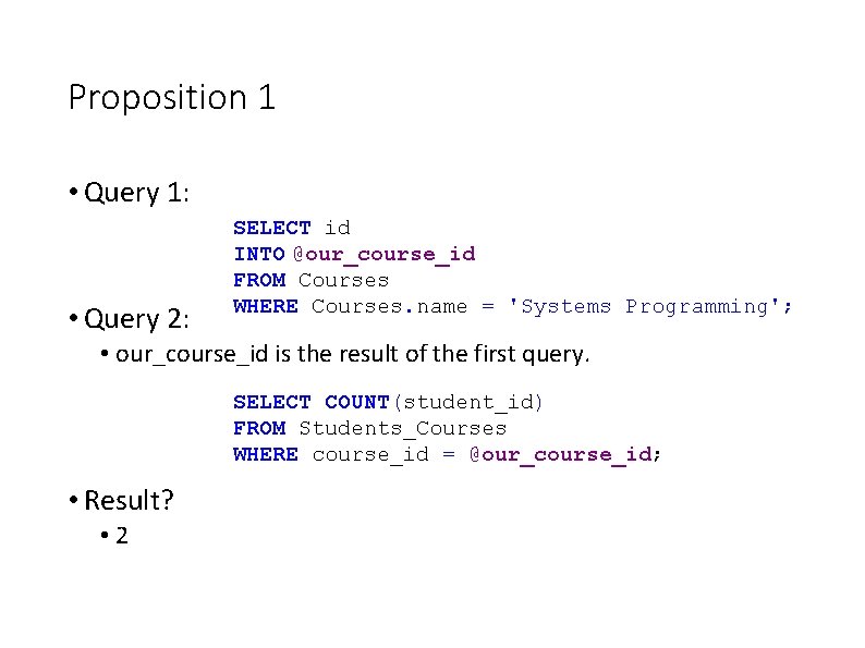
Proposition 1 • Query 1: • Query 2: SELECT id INTO @our_course_id FROM Courses WHERE Courses. name = 'Systems Programming'; • our_course_id is the result of the first query. SELECT COUNT(student_id) FROM Students_Courses WHERE course_id = @our_course_id; • Result? • 2

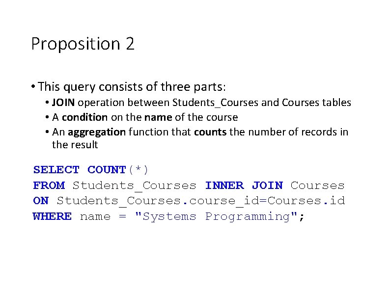
Proposition 2 • This query consists of three parts: • JOIN operation between Students_Courses and Courses tables • A condition on the name of the course • An aggregation function that counts the number of records in the result SELECT COUNT(*) FROM Students_Courses INNER JOIN Courses ON Students_Courses. course_id=Courses. id WHERE name = "Systems Programming";

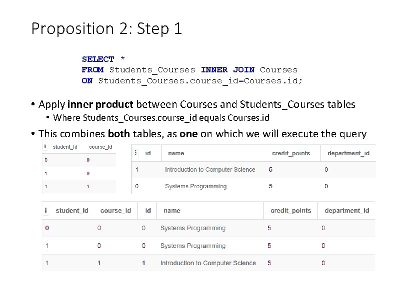
Proposition 2: Step 1 SELECT * FROM Students_Courses INNER JOIN Courses ON Students_Courses. course_id=Courses. id; • Apply inner product between Courses and Students_Courses tables • Where Students_Courses. course_id equals Courses. id • This combines both tables, as one on which we will execute the query

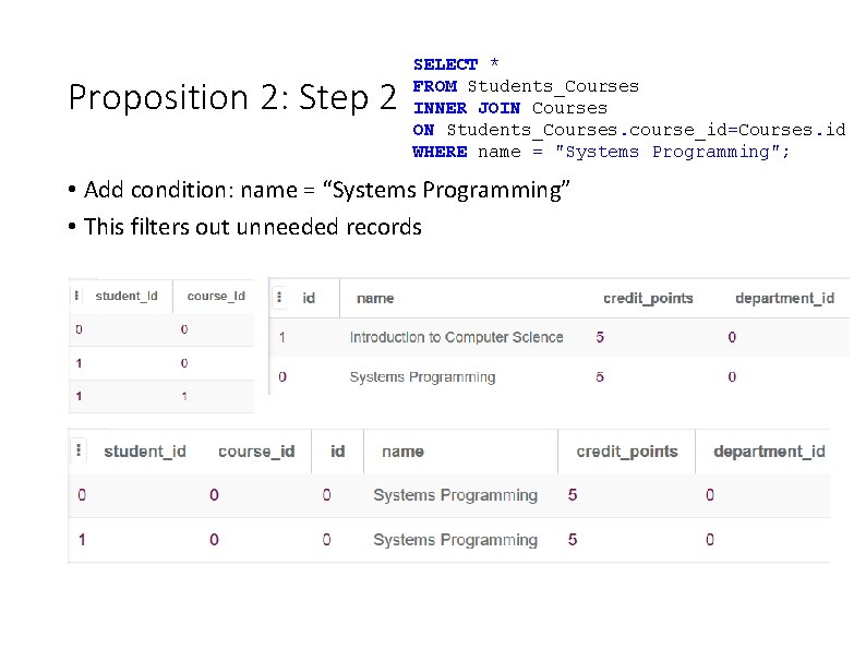
Proposition 2: Step 2 SELECT * FROM Students_Courses INNER JOIN Courses ON Students_Courses. course_id=Courses. id WHERE name = "Systems Programming"; • Add condition: name = “Systems Programming” • This filters out unneeded records

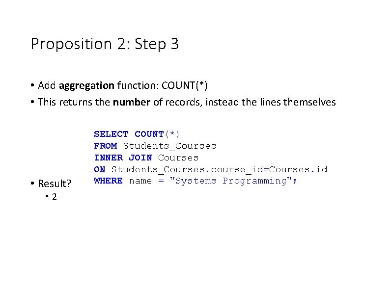
Proposition 2: Step 3 • Add aggregation function: COUNT(*) • This returns the number of records, instead the lines themselves • Result? • 2 SELECT COUNT(*) FROM Students_Courses INNER JOIN Courses ON Students_Courses. course_id=Courses. id WHERE name = "Systems Programming";