Lecture 14 Normal Random Variables IE 360 Design

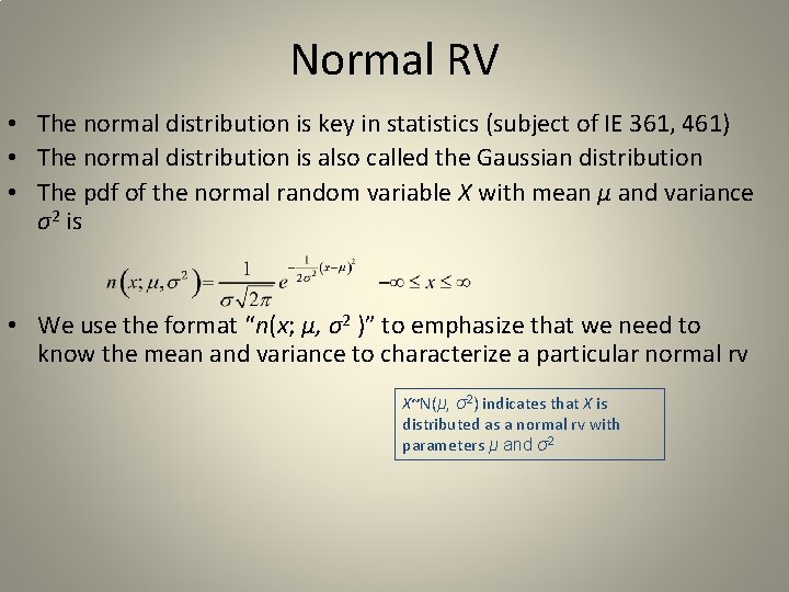
Normal RV • The normal distribution is key in statistics (subject of IE 361, 461) • The normal distribution is also called the Gaussian distribution • The pdf of the normal random variable X with mean μ and variance σ2 is • We use the format “n(x; μ, σ2 )” to emphasize that we need to know the mean and variance to characterize a particular normal rv X~N(μ, σ2) indicates that X is distributed as a normal rv with parameters μ and σ2

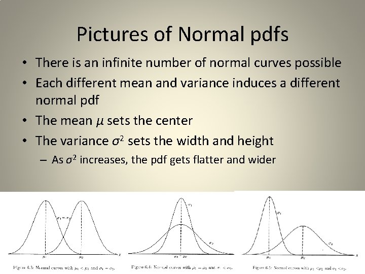
Pictures of Normal pdfs • There is an infinite number of normal curves possible • Each different mean and variance induces a different normal pdf • The mean μ sets the center • The variance σ2 sets the width and height – As σ2 increases, the pdf gets flatter and wider

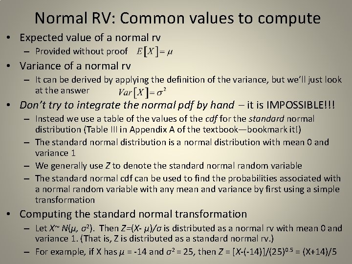
Normal RV: Common values to compute • Expected value of a normal rv – Provided without proof • Variance of a normal rv – It can be derived by applying the definition of the variance, but we’ll just look at the answer • Don’t try to integrate the normal pdf by hand – it is IMPOSSIBLE!!! – Instead we use a table of the values of the cdf for the standard normal distribution (Table III in Appendix A of the textbook—bookmark it!) – The standard normal distribution is a normal distribution with mean 0 and variance 1 – We generally use Z to denote the standard normal random variable – The standard normal cdf can be used to find the probabilities associated with a normal random variable with any mean and variance by first using a simple transformation • Computing the standard normal transformation – Let X~ N(μ, σ2). Then Z=(X- μ)/σ is distributed as a normal rv with mean 0 and variance 1. (That is, Z is distributed as a standard normal rv. ) – For example, if X has μ = -14 and σ2 = 25, then Z = [X-(-14)]/(25)0. 5 = (X+14)/5

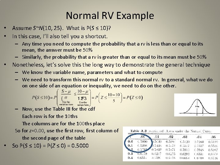
Normal RV Example • Assume S~N(10, 25). What is P(S ≤ 10)? • In this case, I’ll also tell you a shortcut. – Any time you need to compute the probability that a rv is less than or equal to its mean, the answer must be 50% – Similarly, the probability that a rv is greater than or equal to its mean must be 50% • Nonetheless, let’s solve this the long way to demonstrate the general technique – We know the variable name, parameters and what to compute – We need to transform this normal rv to a standard normal rv. In general, what we do on one side of an equation or inequality, we need to do on the other. – Now, use the Table III for the cdf Each row is for the 10 ths The columns are for the 100 ths place So for z=0. 00, use the first row, first column of the second page of the table • So P(S ≤ 10) = P(Z ≤ 0) = 0. 5000

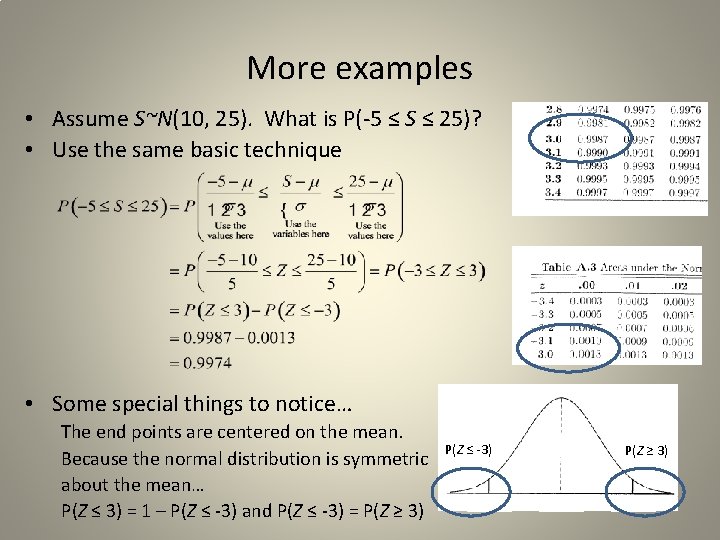
More examples • Assume S~N(10, 25). What is P(-5 ≤ S ≤ 25)? • Use the same basic technique • Some special things to notice… The end points are centered on the mean. Because the normal distribution is symmetric about the mean… P(Z ≤ 3) = 1 – P(Z ≤ -3) and P(Z ≤ -3) = P(Z ≥ 3) P(Z ≤ -3) P(Z ≥ 3)

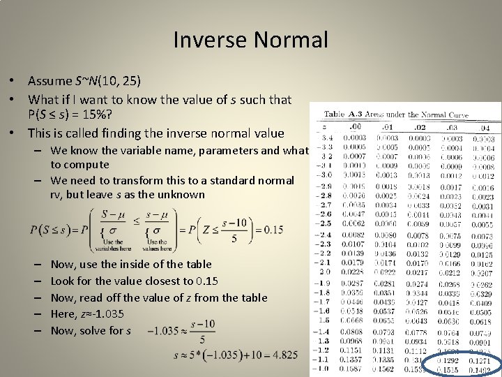
Inverse Normal • Assume S~N(10, 25) • What if I want to know the value of s such that P(S ≤ s) = 15%? • This is called finding the inverse normal value – We know the variable name, parameters and what to compute – We need to transform this to a standard normal rv, but leave s as the unknown – – – Now, use the inside of the table Look for the value closest to 0. 15 Now, read off the value of z from the table Here, z≈-1. 035 Now, solve for s

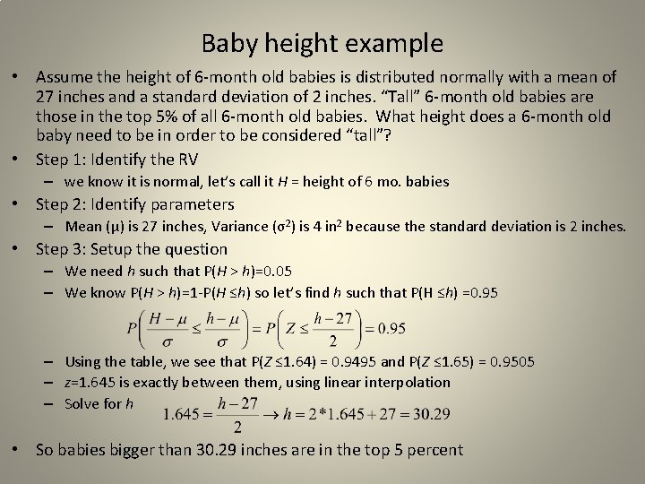
Baby height example • Assume the height of 6 -month old babies is distributed normally with a mean of 27 inches and a standard deviation of 2 inches. “Tall” 6 -month old babies are those in the top 5% of all 6 -month old babies. What height does a 6 -month old baby need to be in order to be considered “tall”? • Step 1: Identify the RV – we know it is normal, let’s call it H = height of 6 mo. babies • Step 2: Identify parameters – Mean (μ) is 27 inches, Variance (σ2) is 4 in 2 because the standard deviation is 2 inches. • Step 3: Setup the question – We need h such that P(H > h)=0. 05 – We know P(H > h)=1 -P(H ≤h) so let’s find h such that P(H ≤h) =0. 95 – Using the table, we see that P(Z ≤ 1. 64) = 0. 9495 and P(Z ≤ 1. 65) = 0. 9505 – z=1. 645 is exactly between them, using linear interpolation – Solve for h • So babies bigger than 30. 29 inches are in the top 5 percent

Related reading • Montgomery and Runger, Sections 4 -6 and 4 -7 • Some links that might help – http: //en. wikipedia. org/wiki/Normal_distribution • Way more info than you probably want – http: //www-stat. stanford. edu/~naras/jsm/Normal. Density. html • More reasonable • Now you are ready to do HW 14