Lecture 14 Interpolating environmental datasets Outline creating surfaces

Lecture 14 Interpolating environmental datasets • Outline – creating surfaces from points – interpolation basics – interpolation methods – common problems Week 17 GEOG 2750 – Earth Observation and GIS of the Physical 1

Introduction • Definition: “Spatial interpolation is the procedure of estimating the values of properties at unsampled sites within an area covered by existing observations. ” (Waters, 1989) • Complex problem – – – Week 17 wide range of applications important in addressing problem of data availability quick fix for partial data coverage interpolation of point data to surface/polygon data role of filling in the gaps between observations GEOG 2750 – Earth Observation and GIS of the Physical 2

Creating surfaces from points • Waters (1989) provides list of potential uses: – – Week 17 to provide contours for displaying data graphically to calculate some property of a surface at a given point to change the unit of comparison when using different data models in different layers to aid in the decision making process both in physical and human geography and in related disciplines such as mineral prospecting and resource evaluation GEOG 2750 – Earth Observation and GIS of the Physical 3

Surfaces from points Points Week 17 Surface GEOG 2750 – Earth Observation and GIS of the Physical 4

An essential skill • Environmental data – often collected as discrete observations at points or along transects – example: soil cores, soil mositure, vegetation transects, meteorological station data, etc. • Need to convert discrete data into continuous surface for use in GIS modelling – interpolation Week 17 GEOG 2750 – Earth Observation and GIS of the Physical 5

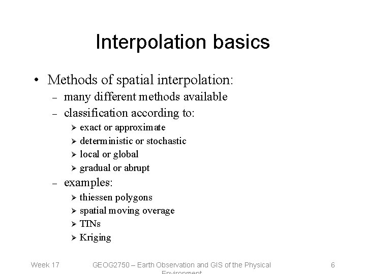
Interpolation basics • Methods of spatial interpolation: – – many different methods available classification according to: exact or approximate Ø deterministic or stochastic Ø local or global Ø gradual or abrupt Ø – examples: thiessen polygons Ø spatial moving overage Ø TINs Ø Kriging Ø Week 17 GEOG 2750 – Earth Observation and GIS of the Physical 6

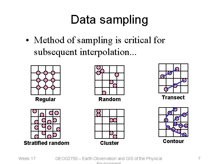
Data sampling • Method of sampling is critical for subsequent interpolation. . . Regular Random Transect Stratified random Cluster Contour Week 17 GEOG 2750 – Earth Observation and GIS of the Physical 7

Question… • How do you choose a method of interpolation? Week 17 GEOG 2750 – Earth Observation and GIS of the Physical 8

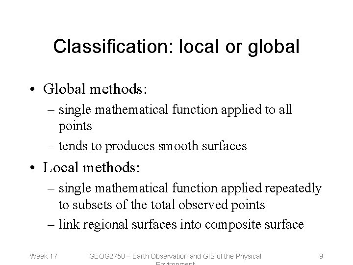
Classification: local or global • Global methods: – single mathematical function applied to all points – tends to produces smooth surfaces • Local methods: – single mathematical function applied repeatedly to subsets of the total observed points – link regional surfaces into composite surface Week 17 GEOG 2750 – Earth Observation and GIS of the Physical 9

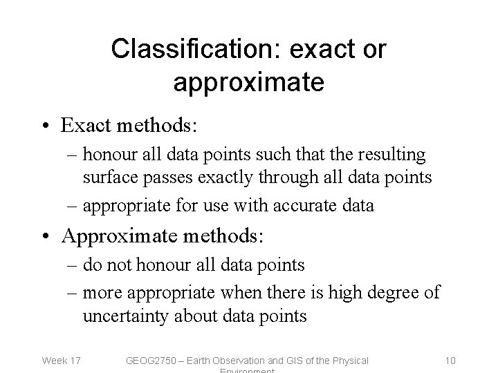
Classification: exact or approximate • Exact methods: – honour all data points such that the resulting surface passes exactly through all data points – appropriate for use with accurate data • Approximate methods: – do not honour all data points – more appropriate when there is high degree of uncertainty about data points Week 17 GEOG 2750 – Earth Observation and GIS of the Physical 10

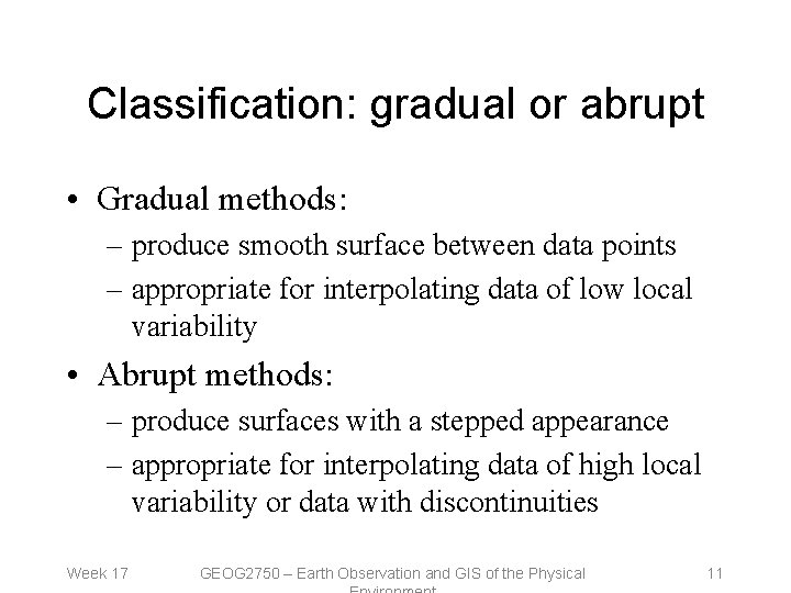
Classification: gradual or abrupt • Gradual methods: – produce smooth surface between data points – appropriate for interpolating data of low local variability • Abrupt methods: – produce surfaces with a stepped appearance – appropriate for interpolating data of high local variability or data with discontinuities Week 17 GEOG 2750 – Earth Observation and GIS of the Physical 11

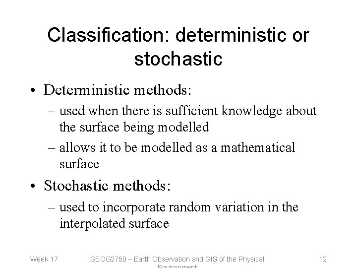
Classification: deterministic or stochastic • Deterministic methods: – used when there is sufficient knowledge about the surface being modelled – allows it to be modelled as a mathematical surface • Stochastic methods: – used to incorporate random variation in the interpolated surface Week 17 GEOG 2750 – Earth Observation and GIS of the Physical 12

Question… • Think of data types that require: – local or global interpolation? – exact or approximate interpolation? – gradual or abrupt interpolation? – deterministic or stochastic interpolation? Week 17 GEOG 2750 – Earth Observation and GIS of the Physical 13

Interpolation methods • Most GIS packages offer a number of methods • Typical methods are: – Thiessen polygons – Triangulated Irregular Networks (TINs) – Spatial moving average – Trend Surfaces Week 17 GEOG 2750 – Earth Observation and GIS of the Physical 14

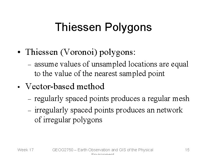
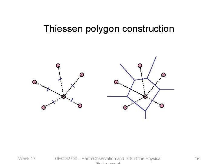
Thiessen Polygons • Thiessen (Voronoi) polygons: – • assume values of unsampled locations are equal to the value of the nearest sampled point Vector-based method – – Week 17 regularly spaced points produces a regular mesh irregularly spaced points produces an network of irregular polygons GEOG 2750 – Earth Observation and GIS of the Physical 15

Thiessen polygon construction Week 17 GEOG 2750 – Earth Observation and GIS of the Physical 16

Example Thiessen polygon Source surface with sample points Week 17 Thiessen polygons with sample points GEOG 2750 – Earth Observation and GIS of the Physical 17

Question… • What categories does the Thiessen polygon method fall into: – – exact or approximate? deterministic or stochastic? gradual or abrupt? local or global? • What could it be used for? Week 17 GEOG 2750 – Earth Observation and GIS of the Physical 18

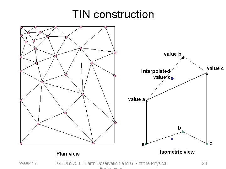
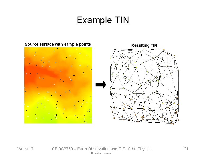
TINs • Another vector-based method often used to create digital terrain models (DTMs) – adjacent data points connected by lines (vertices) to create a network of irregular triangles Ø calculate real 3 D distance between data points along vertices using trigonometry Ø calculate interpolated value along facets between three vertices Week 17 GEOG 2750 – Earth Observation and GIS of the Physical 19

TIN construction value b value c Interpolated value x value a b c a Plan view Week 17 Isometric view GEOG 2750 – Earth Observation and GIS of the Physical 20

Example TIN Source surface with sample points Week 17 Resulting TIN GEOG 2750 – Earth Observation and GIS of the Physical 21

Question… • What categories does the TIN method fall into: – – exact or approximate? deterministic or stochastic? gradual or abrupt? local or global? • What could it be used for? Week 17 GEOG 2750 – Earth Observation and GIS of the Physical 22

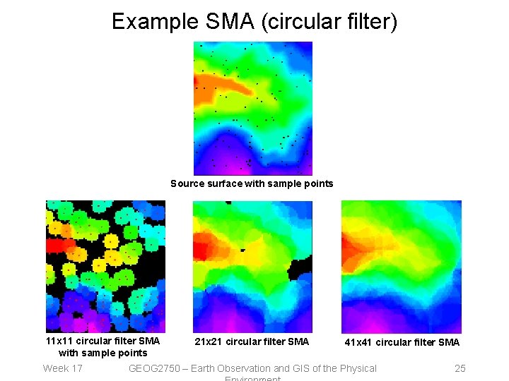
Spatial moving average • Vector and raster method: – – – most common GIS method calculates new value of each location based on range of values associated with neighbouring points Neighbourhood determined by a filter Ø size, Week 17 shape and character of filter? GEOG 2750 – Earth Observation and GIS of the Physical 23

Spatial moving average (SMA) Week 17 GEOG 2750 – Earth Observation and GIS of the Physical 24

Example SMA (circular filter) Source surface with sample points 11 x 11 circular filter SMA with sample points Week 17 21 x 21 circular filter SMA 41 x 41 circular filter SMA GEOG 2750 – Earth Observation and GIS of the Physical 25

Question… • What categories does the SMA method fall into: – – exact or approximate? deterministic or stochastic? gradual or abrupt? local or global? • What could it be used for? Week 17 GEOG 2750 – Earth Observation and GIS of the Physical 26

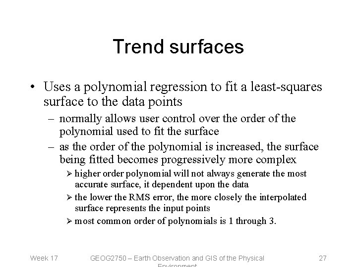
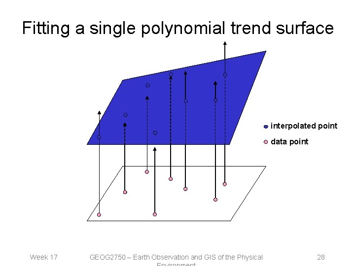
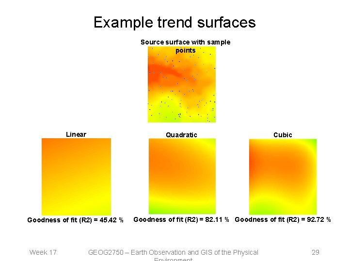
Trend surfaces • Uses a polynomial regression to fit a least-squares surface to the data points – normally allows user control over the order of the polynomial used to fit the surface – as the order of the polynomial is increased, the surface being fitted becomes progressively more complex Ø higher order polynomial will not always generate the most accurate surface, it dependent upon the data Ø the lower the RMS error, the more closely the interpolated surface represents the input points Ø most common order of polynomials is 1 through 3. Week 17 GEOG 2750 – Earth Observation and GIS of the Physical 27

Fitting a single polynomial trend surface interpolated point data point Week 17 GEOG 2750 – Earth Observation and GIS of the Physical 28

Example trend surfaces Source surface with sample points Linear Quadratic Goodness of fit (R 2) = 45. 42 % Week 17 Cubic Goodness of fit (R 2) = 82. 11 % Goodness of fit (R 2) = 92. 72 % GEOG 2750 – Earth Observation and GIS of the Physical 29

Question… • What categories does the trend surface method fall into: – – exact or approximate? deterministic or stochastic? gradual or abrupt? local or global? • What could it be used for? Week 17 GEOG 2750 – Earth Observation and GIS of the Physical 30

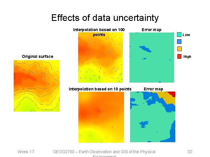
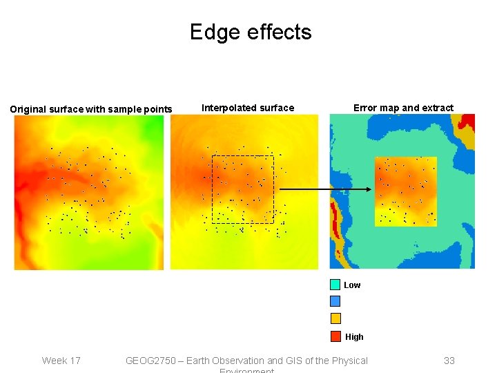
Common problems • Input data uncertainty – Too few data points – Limited or clustered spatial coverage – Uncertainty about location and/or value • Edge effects – Need data points outside study area – improve interpolation and avoid distortion at boundaries Week 17 GEOG 2750 – Earth Observation and GIS of the Physical 31

Effects of data uncertainty Interpolation based on 100 points Error map Low Original surface High Interpolation based on 10 points Week 17 Error map GEOG 2750 – Earth Observation and GIS of the Physical 32

Edge effects Original surface with sample points Interpolated surface Error map and extract Low High Week 17 GEOG 2750 – Earth Observation and GIS of the Physical 33

Question… • Is it possible to use explanatory variables to improve interpolation, and if so, how? Week 17 GEOG 2750 – Earth Observation and GIS of the Physical 34

Conclusions • Interpolation of environmental point data is important skill • Many methods classified by – local/global, approximate/exact, gradual/abrupt and deterministic/stochastic – choice of method is crucial to success • Error and uncertainty – poor input data – poor choice/implementation of interpolation method Week 17 GEOG 2750 – Earth Observation and GIS of the Physical 35

Practical • Interpolating surfaces from point data • Task: Interpolate a selection of point data using the most appropriate methods of your choosing • Data: The following datasets are provided for the Yorkshire area… – 200 m resolution DEM (derived from 1: 50, 000 OS Panorama data) – 25 m interval contour data (derived from 1: 50, 000 OS Panorama data) – metstation data (mean annual rainfall) Week 17 GEOG 2750 – Earth Observation and GIS of the Physical 36

Practical • Steps: 1. Look at the data carefully and choose appropriate technique(s) for interpolating rainfall– which is most appropriate and why? 2. Interpolate rainfall data using chosen method(s) – have you chosen more than one method and if so why? 3. Display the resulting surface – does it look right, if not why? Week 17 GEOG 2750 – Earth Observation and GIS of the Physical 37

Learning outcomes • Familiarisation with range of different interpolation techniques • Experience at applying interpolation methods in Arc and Arc. GRID to environmental datasets Week 17 GEOG 2750 – Earth Observation and GIS of the Physical 38

Useful web links • Another 2 lectures on interpolation – http: //www. geog. ubc. ca/courses/klink/gis. notes/ncgia/u 40. html – http: //www. geog. ubc. ca/courses/klink/gis. notes/ncgia/u 41. html Week 17 GEOG 2750 – Earth Observation and GIS of the Physical 39

Next week… • Principles of grid-based modelling – linking models to GIS – basics of cartographic modelling – modelling in Arc. GRID • Practical: Land Capability Mapping Week 17 GEOG 2750 – Earth Observation and GIS of the Physical 40