Lecture 14 Graph Algorithms ShangHua Teng Undirected Graphs

Lecture 14: Graph Algorithms Shang-Hua Teng

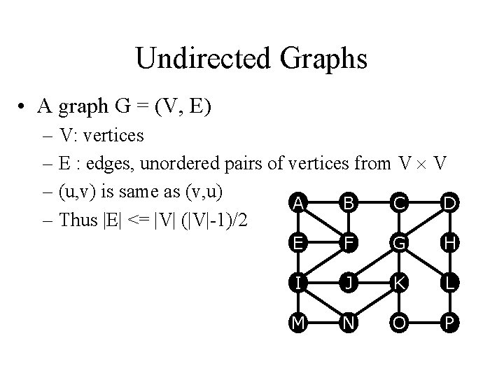
Undirected Graphs • A graph G = (V, E) – V: vertices – E : edges, unordered pairs of vertices from V V – (u, v) is same as (v, u) A B C D – Thus |E| <= |V| (|V|-1)/2 E F G H I J K L M N O P

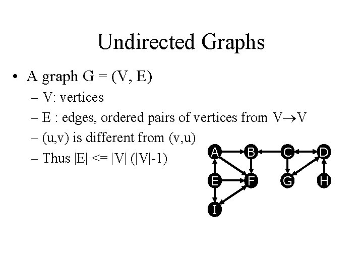
Undirected Graphs • A graph G = (V, E) – V: vertices – E : edges, ordered pairs of vertices from V V – (u, v) is different from (v, u) A B C D – Thus |E| <= |V| (|V|-1) E I F G H

Basic Graph Properties • An undirected graph is connected if it has a path from every vertex to every other • A directed graph is strongly connected if it has a path from every vertex to every other • A weighted graph associates weights with either the edges or the vertices • E. g. , a road map: edges might be weighted w/ distance • A multigraph allows multiple edges between the same vertices

Dense and Sparse Graphs • We will typically express running times in terms of |E| and |V| (often dropping the |’s) – If |E| |V|2 the graph is dense – If |E| |V| the graph is sparse • Different data structures may be used to express sparse and dense graph

Graph in Applications • Internet: web graphs – Each page is a vertex – Each edge represent a hyperlink – Directed • GPS: highway maps – Each city is a vertex – Each freeway segment is an undirected edge – Undirected • Graphs are ubiquitous in computer science

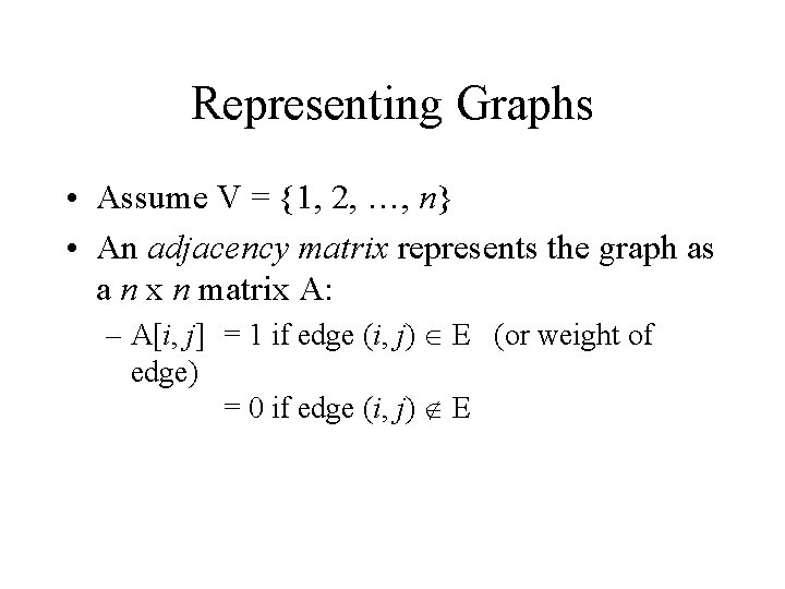
Representing Graphs • Assume V = {1, 2, …, n} • An adjacency matrix represents the graph as a n x n matrix A: – A[i, j] = 1 if edge (i, j) E (or weight of edge) = 0 if edge (i, j) E

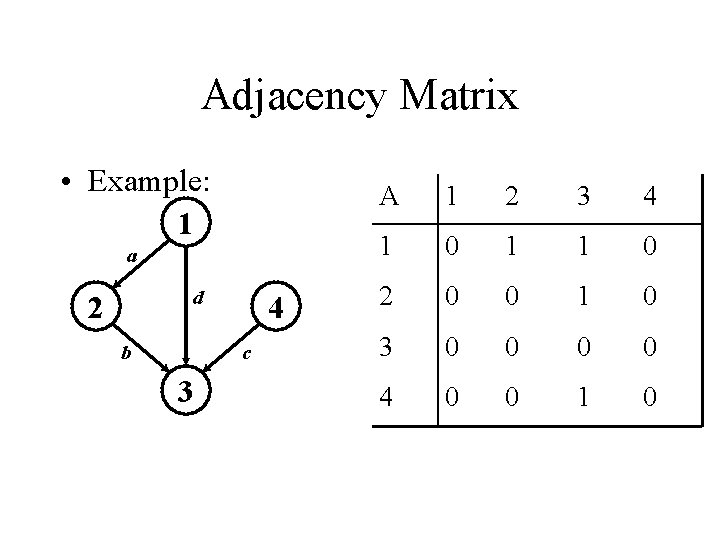
Adjacency Matrix • Example: 1 a d 2 b 4 c 3 A 1 2 3 4 1 0 1 1 0 2 0 0 1 0 3 0 0 4 0 0 1 0

Adjacency Matrix Representation • Undirected graph matrix A is symmetric • Storage requirements: O(V 2) – A dense representation • The adjacency matrix is a dense representation – Usually too much storage for large graphs – But can be very efficient for small graphs • Most large interesting graphs are sparse – For example, trees and planar graphs (such as highway map) have |E| = O(|V|) – For this reason, we often needs more sparse representation

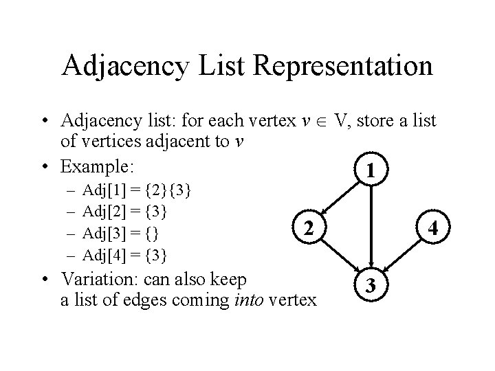
Adjacency List Representation • Adjacency list: for each vertex v V, store a list of vertices adjacent to v • Example: 1 – – Adj[1] = {2}{3} Adj[2] = {3} Adj[3] = {} Adj[4] = {3} 2 • Variation: can also keep a list of edges coming into vertex 4 3

Adjacency List Representation • The degree of a vertex v in an undirected graph is equal to the number of incident edges • For directed graphs, we can define in-degree, out-degree for each vertex • For directed graphs, the total size of the adjacency lists is out-degree(v) = |E| takes (V + E) storage • For undirected graphs, the total size of the adjacent lists is degree(v) = 2 |E| also (V + E) storage • So: Adjacency lists take O(V+E) storage

Google Problem: Graph Searching • How to search and explore in the Web Space? • How to find all web-pages and all the hyperlinks? – Start from one vertex “www. google. com” – Systematically follow hyperlinks from the discovered vertex/web page – Build a search tree along the exploration

General Graph Searching • Input: a graph G = (V, E), directed or undirected • Objective: methodically explore every vertex and every edge • Build a tree on the graph – Pick a vertex as the root – Choose certain edges to produce a tree – Note: might also build a forest if graph is not connected

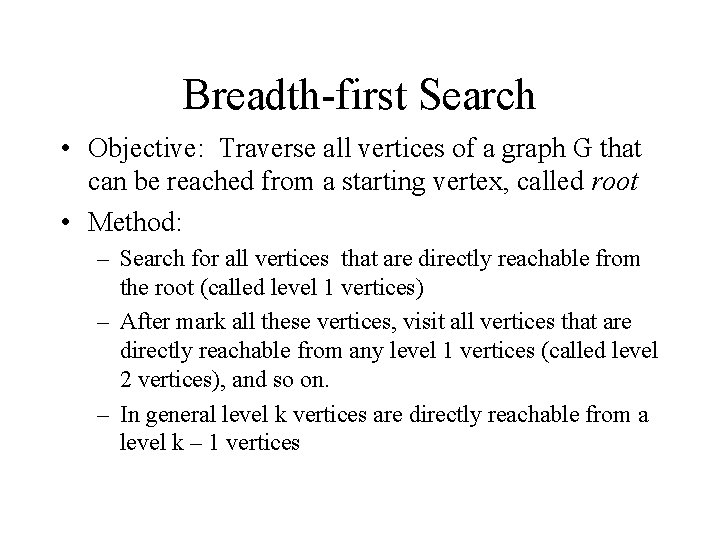
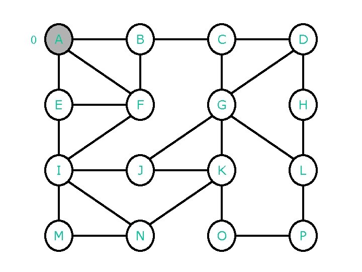
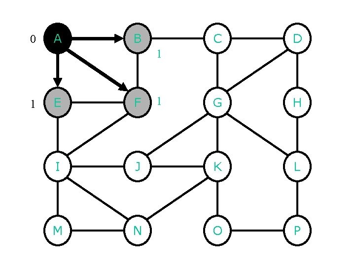
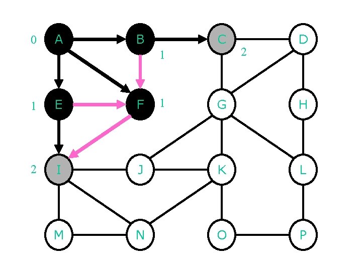
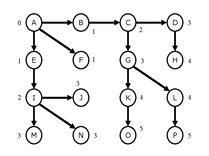
Breadth-first Search • Objective: Traverse all vertices of a graph G that can be reached from a starting vertex, called root • Method: – Search for all vertices that are directly reachable from the root (called level 1 vertices) – After mark all these vertices, visit all vertices that are directly reachable from any level 1 vertices (called level 2 vertices), and so on. – In general level k vertices are directly reachable from a level k – 1 vertices

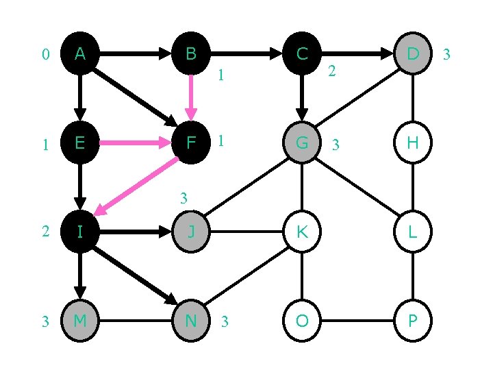
An Example

0 A B C D E F G H I J K L M N O P

0 A B C D G H 1 1 1 E F I J K L M N O P

0 A B C 1 1 E F 2 I M 1 2 D G H J K L N O P

0 A B C 1 1 E F 1 G 2 3 D H 3 2 I J 3 M N 3 K L O P 3

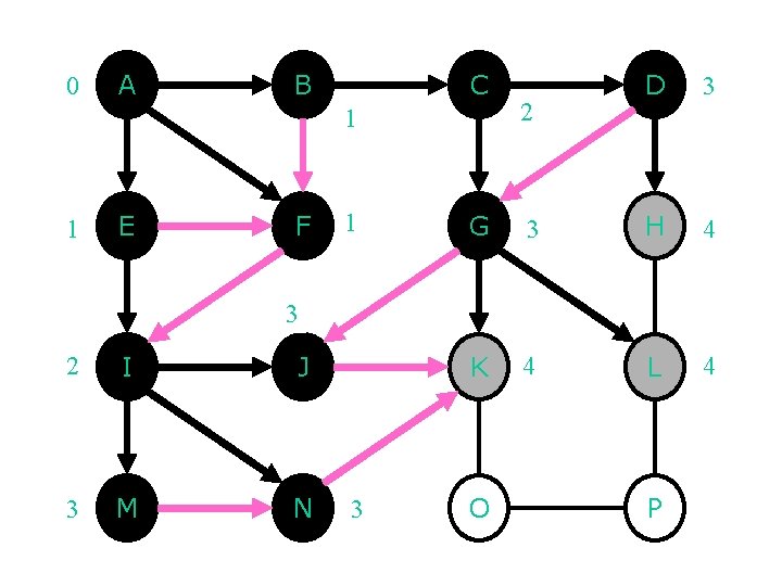
0 A B C 1 1 E F 1 2 D 3 G 3 H 4 K 4 L 4 3 2 I J 3 M N 3 O P

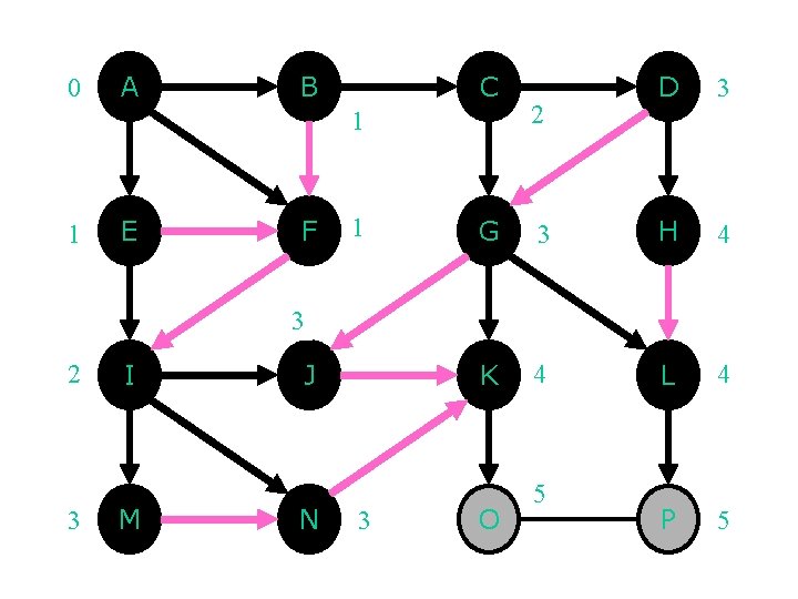
0 A B C 1 1 E F 1 2 D 3 G 3 H 4 K 4 L 4 P 5 3 2 3 I M J N 3 O 5

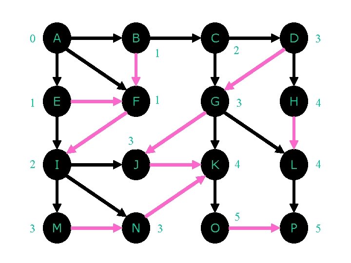
0 A B C 1 1 E F 1 2 D 3 G 3 H 4 K 4 L 4 P 5 3 2 3 I M J N 3 O 5

0 A B C 1 1 E F 1 2 D 3 G 3 H 4 K 4 L 4 P 5 3 2 3 I M J N 3 O 5

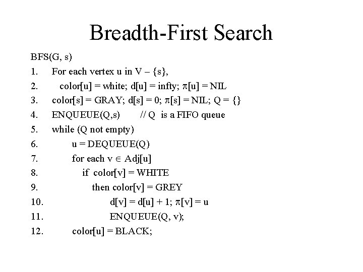
Breadth-First Search BFS(G, s) 1. For each vertex u in V – {s}, 2. color[u] = white; d[u] = infty; p[u] = NIL 3. color[s] = GRAY; d[s] = 0; p[s] = NIL; Q = {} 4. ENQUEUE(Q, s) // Q is a FIFO queue 5. while (Q not empty) 6. u = DEQUEUE(Q) 7. for each v Adj[u] 8. if color[v] = WHITE 9. then color[v] = GREY 10. d[v] = d[u] + 1; p[v] = u 11. ENQUEUE(Q, v); 12. color[u] = BLACK;

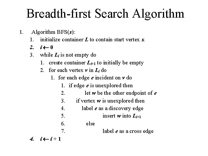
Breadth-first Search Algorithm 1. Algorithm BFS(s): 1. initialize container L to contain start vertex s. 2. i 0 3. while Li is not empty do 1. create container Li+1 to initially be empty 2. for each vertex v in Li do 1. for each edge e incident on v do 1. if edge e is unexplored then 2. let w be the other endpoint of e 3. if vertex w is unexplored then 4. label e as a discovery edge 5. insert w into Li+1 6. else 7. label e as a cross edge 4. i i + 1

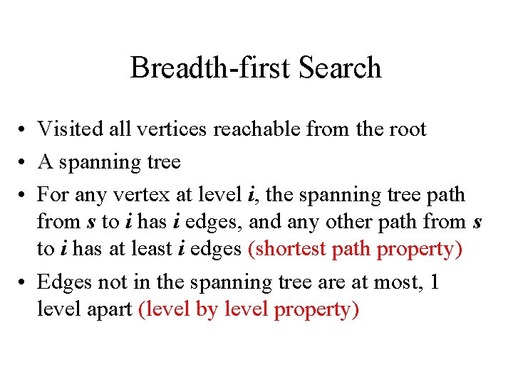
Breadth-first Search • Visited all vertices reachable from the root • A spanning tree • For any vertex at level i, the spanning tree path from s to i has i edges, and any other path from s to i has at least i edges (shortest path property) • Edges not in the spanning tree are at most, 1 level apart (level by level property)

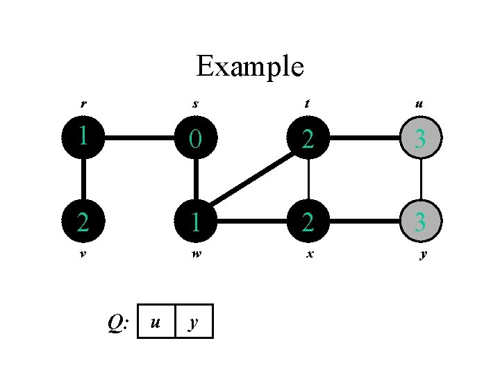
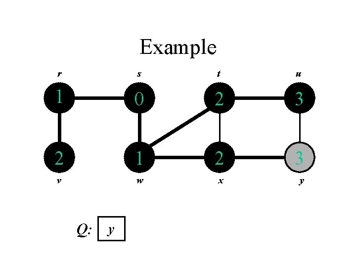
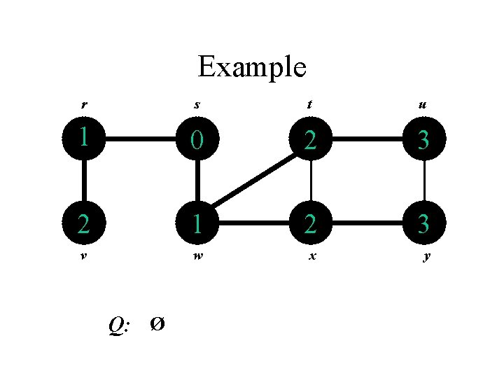
Breadth-First Search: the Color Scheme • White vertices have not been discovered – All vertices start out white • Grey vertices are discovered but not fully explored – They may be adjacent to white vertices • Black vertices are discovered and fully explored – They are adjacent only to black and gray vertices • Explore vertices by scanning adjacency list of grey vertices

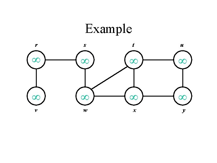
Example r s t u v w x y

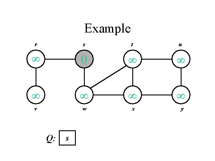
Example r s t u 0 v w x y Q: s

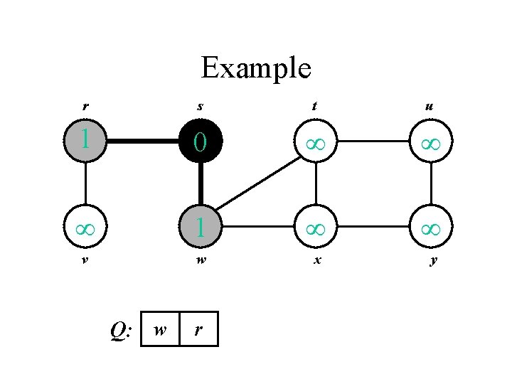
Example r s t u 1 0 1 v w x y Q: w r

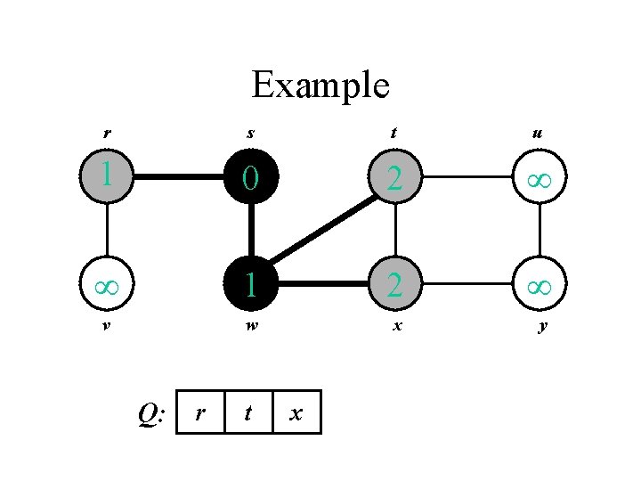
Example r s t u 1 0 2 1 2 v w x y Q: r t x

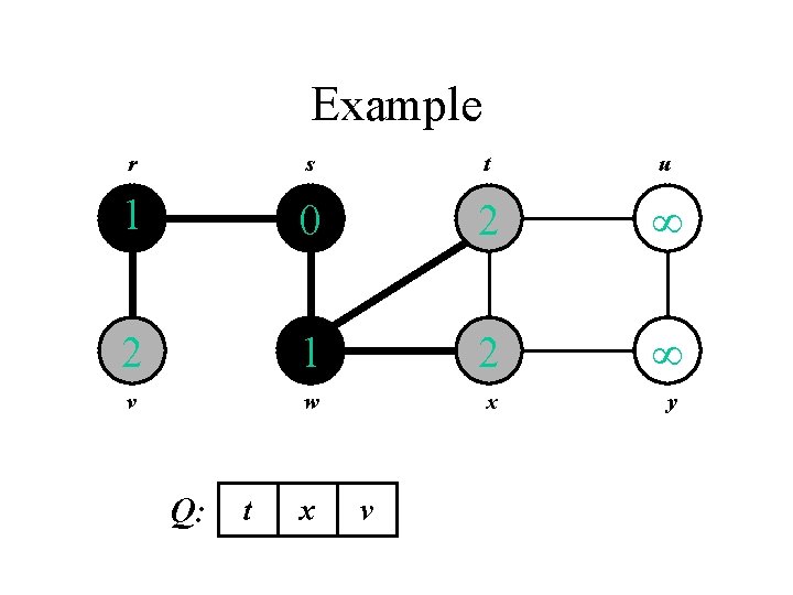
Example r s t u 1 0 2 2 1 2 v w x y Q: t x v

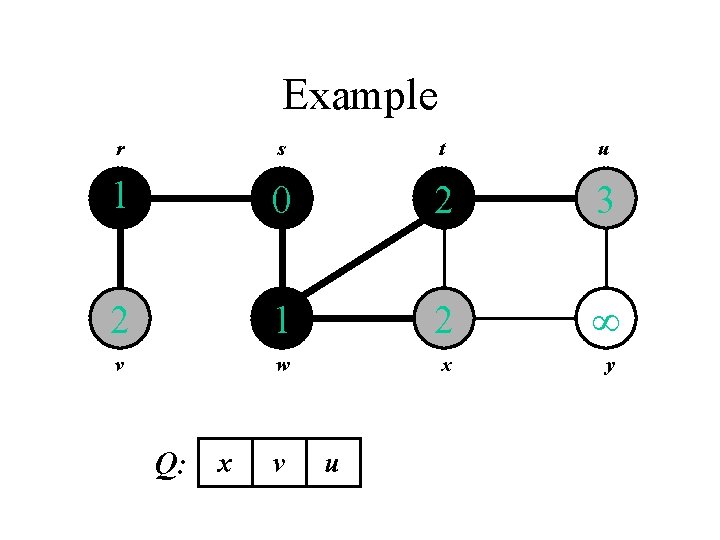
Example r s t u 1 0 2 3 2 1 2 v w x y Q: x v u

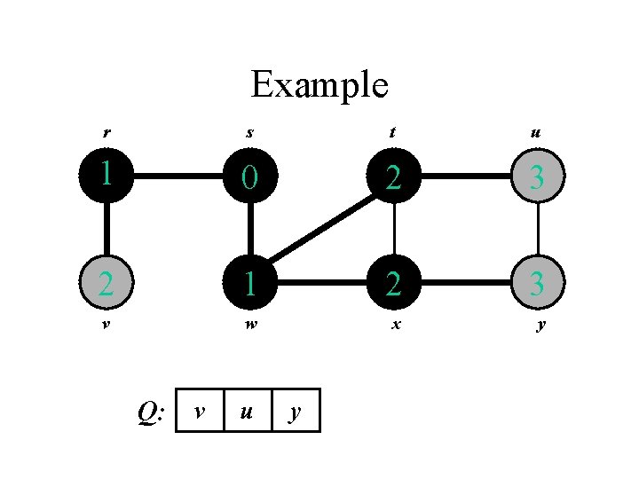
Example r s t u 1 0 2 3 2 1 2 3 v w x y Q: v u y

Example r s t u 1 0 2 3 2 1 2 3 v w x y Q: u y

Example r s t u 1 0 2 3 2 1 2 3 v w x y Q: y

Example r s t u 1 0 2 3 2 1 2 3 v w x y Q: Ø

Properties of BFS • BFS calculates the shortest-path distance to the source node – Shortest-path distance (s, v) = minimum number of edges from s to v, or if v not reachable from s – Prove using blackboard • BFS builds breadth-first tree, in which paths to root represent shortest paths in G – Thus can use BFS to calculate shortest path from one vertex to another in O(V+E) time

Properties of BFS • Proposition: Let G be an undirected graph on which a BFS traversal starting at vertex s has been performed. Then – The traversal visits all vertices in the connected component of s. – The discovery-edges form a spanning tree T, which we call the BFS tree, of the connected component of s – For each vertex v at level i, the path of the BFS tree T between s and v has i edges, and any other path of G between s and v has at least i edges. – If (u, v) is an edge that is not in the BFS tree, then the level numbers of u and v differ by at most one. 39

Properties of BFS • Proposition: Let G be a graph with n vertices and m edges. A BFS traversal of G takes time O(n + m). Also, there exist O(n + m) time algorithms based on BFS for the following problems: – Testing whether G is connected. – Computing a spanning tree of G – Computing the connected components of G – Computing, for every vertex v of G, the minimum number of edges of any path between s and v. 40