Lecture 13 Specific Continuous Random Variables IE 360

Lecture 13 Specific Continuous Random Variables IE 360: Design and Control of Industrial Systems I References Montgomery and Runger Sections 4 -5, 4 -8 Copyright 2010 by Joel Greenstein
Why look at some specific continuous rvs? • For the same reasons as for the discrete case – We can develop some short cuts that will be useful in general – We can always derive pdfs, but some of them come up over and over again in asking some questions • We can abstract out the common elements of these stories and derive pdfs that work in general • We will look at 3 specific continuous random variables – Continuous uniform • It is easy and a good ramp-up – Exponential • It is related to the Poisson RV • Stochastic OR (IE 381 and parts of IE 482) is built on it – Normal • Statistics in general (IE 361 and IE 461) is built on it
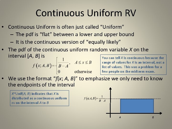
Continuous Uniform RV • Continuous Uniform is often just called “Uniform” – The pdf is “flat” between a lower and upper bound – It is the continuous version of “equally likely” • The pdf of the continuous uniform random variable X on the interval [A, B] is You can tell X is continuous because the range of values for X is an interval, not a list of values. This was a problem for a few people on the midterm exam. • We use the format “f(x; A, B)” to emphasize we only need to know the endpoints of the interval X~Unif(A, B) indicates that X is distributed as a continuous uniform rv on the interval A to B A B
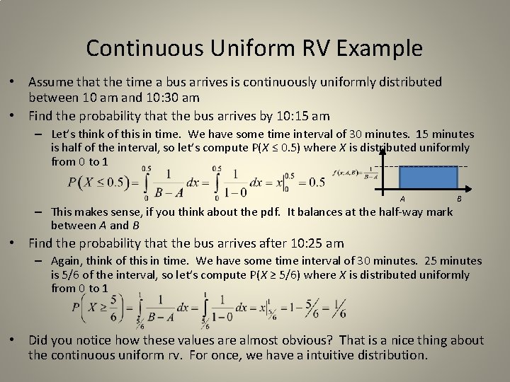
Continuous Uniform RV Example • Assume that the time a bus arrives is continuously uniformly distributed between 10 am and 10: 30 am • Find the probability that the bus arrives by 10: 15 am – Let’s think of this in time. We have some time interval of 30 minutes. 15 minutes is half of the interval, so let’s compute P(X ≤ 0. 5) where X is distributed uniformly from 0 to 1 A – This makes sense, if you think about the pdf. It balances at the half-way mark between A and B B • Find the probability that the bus arrives after 10: 25 am – Again, think of this in time. We have some time interval of 30 minutes. 25 minutes is 5/6 of the interval, so let’s compute P(X ≥ 5/6) where X is distributed uniformly from 0 to 1 • Did you notice how these values are almost obvious? That is a nice thing about the continuous uniform rv. For once, we have a intuitive distribution.

Continuous Uniform RV: common values to compute • Expected value of a Continuous Uniform rv – Just apply the definition of expected value with the general pdf • Is that what you would expect, based on the “balancing” interpretation of the expected value? • Variance of a Continuous Uniform rv – Again, just apply the definition of variance, we’ll just look at the answer

Exponential RV • The exponential distribution is key in Stochastic OR (IE 381) • The pdf of the exponential random variable X with parameter λ • is • We use the format “f(x; λ)” to emphasize we only need to know the parameter λ X~Exp(λ) indicates that X is distributed as an exponential rv on with parameter λ The pdf starts at λ and then falls at a constant rate, never hitting but approaching zero.
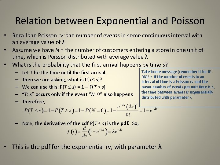
Relation between Exponential and Poisson • Recall the Poisson rv: the number of events in some continuous interval with an average value of λ • Assume we have N = the number of customers entering a store in one unit of time, which is Poisson distributed with average value λ • What is the probability that the first arrival happens by time s? – – – Let T be the time until the first arrival. Then we are asking, what is P(T≤ s)? We can use this: P(T ≤ s) = 1 – P(T > s) “T>s” occurs only if the event “N=0” also happens Therefore, Take home message (remember it for IE 381!): If the number of events in an interval of time is a Poisson rv and the mean number of events per unit time is λ, the time between events is exponentially distributed with parameter λ – Now, the derivative of the cdf P(T ≤ s) is the pdf. So, • This is the pdf for the exponential rv, with parameter λ
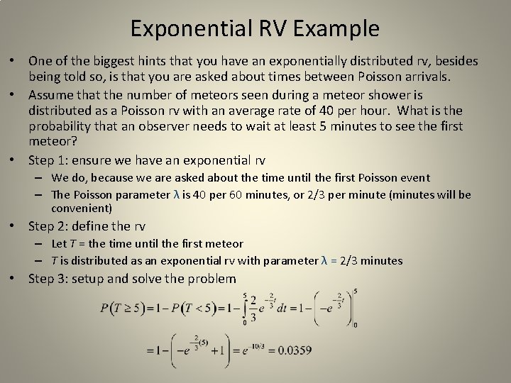
Exponential RV Example • One of the biggest hints that you have an exponentially distributed rv, besides being told so, is that you are asked about times between Poisson arrivals. • Assume that the number of meteors seen during a meteor shower is distributed as a Poisson rv with an average rate of 40 per hour. What is the probability that an observer needs to wait at least 5 minutes to see the first meteor? • Step 1: ensure we have an exponential rv – We do, because we are asked about the time until the first Poisson event – The Poisson parameter λ is 40 per 60 minutes, or 2/3 per minute (minutes will be convenient) • Step 2: define the rv – Let T = the time until the first meteor – T is distributed as an exponential rv with parameter λ = 2/3 minutes • Step 3: setup and solve the problem
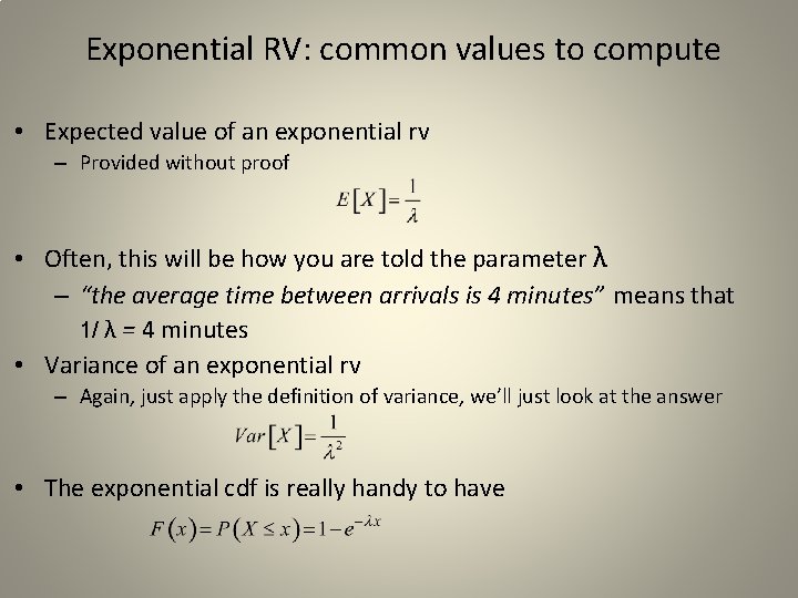
Exponential RV: common values to compute • Expected value of an exponential rv – Provided without proof • Often, this will be how you are told the parameter λ – “the average time between arrivals is 4 minutes” means that 1/ λ = 4 minutes • Variance of an exponential rv – Again, just apply the definition of variance, we’ll just look at the answer • The exponential cdf is really handy to have
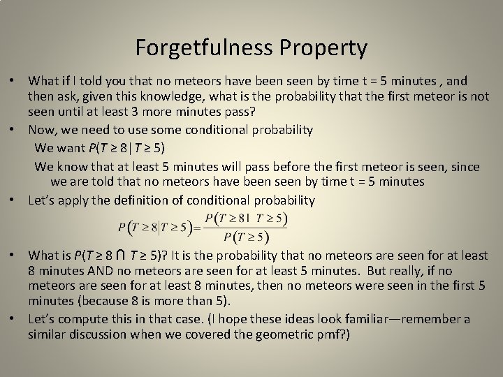
Forgetfulness Property • What if I told you that no meteors have been seen by time t = 5 minutes , and then ask, given this knowledge, what is the probability that the first meteor is not seen until at least 3 more minutes pass? • Now, we need to use some conditional probability We want P(T ≥ 8|T ≥ 5) We know that at least 5 minutes will pass before the first meteor is seen, since we are told that no meteors have been seen by time t = 5 minutes • Let’s apply the definition of conditional probability • What is P(T ≥ 8 ∩ T ≥ 5)? It is the probability that no meteors are seen for at least 8 minutes AND no meteors are seen for at least 5 minutes. But really, if no meteors are seen for at least 8 minutes, then no meteors were seen in the first 5 minutes (because 8 is more than 5). • Let’s compute this in that case. (I hope these ideas look familiar—remember a similar discussion when we covered the geometric pmf? )
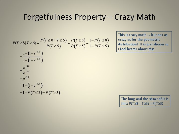
Forgetfulness Property – Crazy Math This is crazy math … but not as crazy as for the geometric distribution! It is just shown so I feel better about this. The long and the short of it is this: P(T≥ 8 | T≥ 5) = P(T≥ 3)
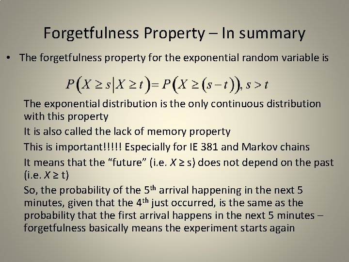
Forgetfulness Property – In summary • The forgetfulness property for the exponential random variable is The exponential distribution is the only continuous distribution with this property It is also called the lack of memory property This is important!!!!! Especially for IE 381 and Markov chains It means that the “future” (i. e. X ≥ s) does not depend on the past (i. e. X ≥ t) So, the probability of the 5 th arrival happening in the next 5 minutes, given that the 4 th just occurred, is the same as the probability that the first arrival happens in the next 5 minutes – forgetfulness basically means the experiment starts again
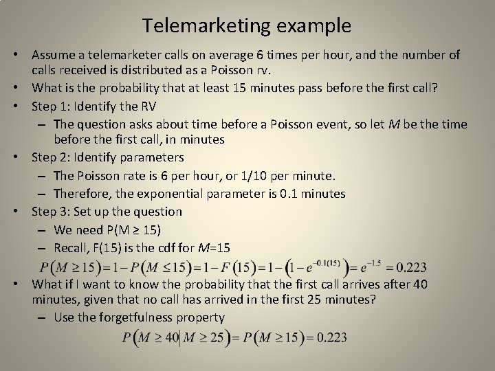
Telemarketing example • Assume a telemarketer calls on average 6 times per hour, and the number of calls received is distributed as a Poisson rv. • What is the probability that at least 15 minutes pass before the first call? • Step 1: Identify the RV – The question asks about time before a Poisson event, so let M be the time before the first call, in minutes • Step 2: Identify parameters – The Poisson rate is 6 per hour, or 1/10 per minute. – Therefore, the exponential parameter is 0. 1 minutes • Step 3: Set up the question – We need P(M ≥ 15) – Recall, F(15) is the cdf for M=15 • What if I want to know the probability that the first call arrives after 40 minutes, given that no call has arrived in the first 25 minutes? – Use the forgetfulness property
Related reading • Montgomery and Runger, Sections 4 -5 and 4 -8 • Some links that might help – http: //en. wikipedia. org/wiki/Exponential_distribution – http: //www. math. uah. edu/stat/index. xhtml • Keep this one – it is really good!!!! It may even help in IE 381 • Now you are ready to do HW 13
- Slides: 14