Lecture 13 Introduction to Time Series John Rundle

Lecture 13 Introduction to Time Series John Rundle Econophysics PHYS 250

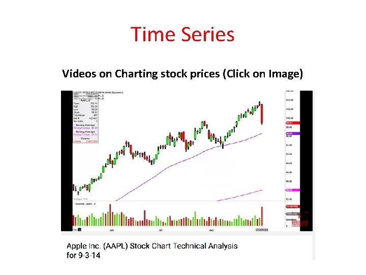
Time Series Videos on Charting stock prices (Click on Image)

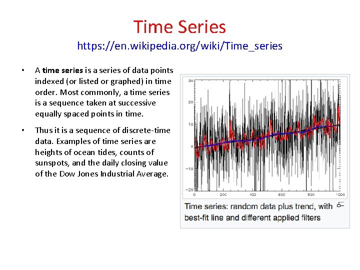
Time Series https: //en. wikipedia. org/wiki/Time_series • A time series is a series of data points indexed (or listed or graphed) in time order. Most commonly, a time series is a sequence taken at successive equally spaced points in time. • Thus it is a sequence of discrete-time data. Examples of time series are heights of ocean tides, counts of sunspots, and the daily closing value of the Dow Jones Industrial Average.

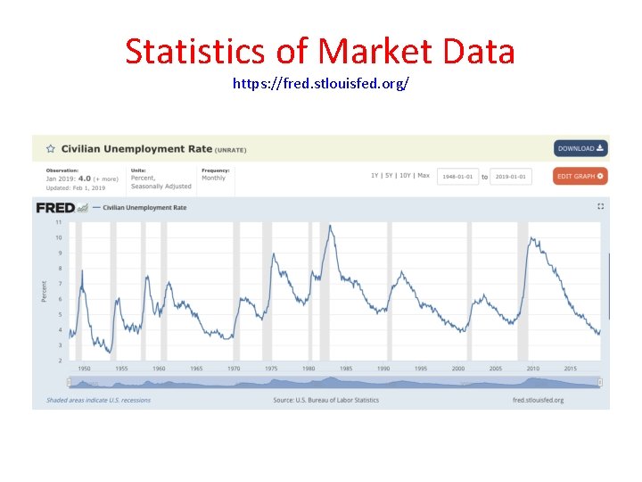
Statistics of Market Data https: //fred. stlouisfed. org/

Time Series https: //en. wikipedia. org/wiki/Time_series • Time series are used in statistics, signal processing, pattern recognition, econometrics, mathematical finance, weather forecasting, intelligent transport and trajectory forecasting, earthquake prediction, electroencephalography, control engineering, astronomy, communications engineering, and largely in any domain of applied science and engineering which involves temporal measurements. • Time series analysis comprises methods for analyzing time series data in order to extract meaningful statistics and other characteristics of the data. • Time series forecasting is the use of a model to predict future values based on previously observed values. • “Time series analysis”, focuses on comparing values of a single time series or multiple dependent time series at different points in time.

Time Series https: //en. wikipedia. org/wiki/Time_series • Methods for time series analysis may be divided into two classes: frequency-domain methods and time-domain methods. • The former include spectral analysis and wavelet analysis • The latter include auto-correlation and cross-correlation analysis. • Time series analysis techniques may be divided into parametric and non-parametric methods. • The parametric approaches assume that the underlying stationary stochastic process has a certain structure which can be described using a small number of parameters (for example, using an autoregressive or moving average model). • In these approaches, the task is to estimate the parameters of the model that describes the stochastic process. • By contrast, non-parametric approaches explicitly estimate the covariance or the spectrum of the process without assuming that the process has any particular structure.

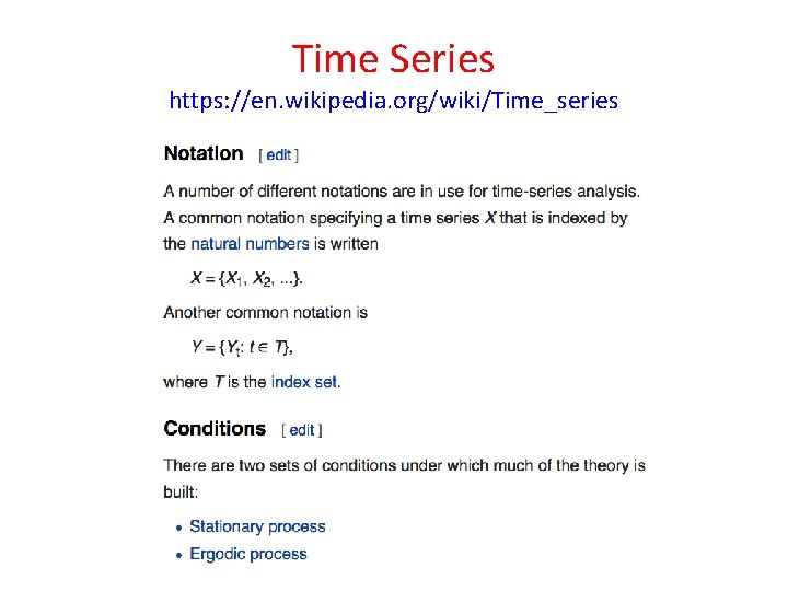
Time Series https: //en. wikipedia. org/wiki/Time_series

Time Series https: //en. wikipedia. org/wiki/Time_series Models • Models for time series data can have many forms and represent different stochastic processes. • When modeling variations in the level of a process, three broad classes of practical importance are the autoregressive (AR) models, the integrated (I) models, and the moving average (MA) models. • These three classes depend linearly on previous data points. • Combinations of these ideas produce autoregressive moving average (ARMA) and autoregressive integrated moving average (ARIMA) models. • The autoregressive fractionally integrated moving average (ARFIMA) model generalizes the former three. • Non-linear dependence of the level of a series on previous data points is of interest, partly because of the possibility of producing a chaotic time series.

Time Series https: //en. wikipedia. org/wiki/Time_series • Among other types of non-linear time series models, there are models to represent the changes of variance over time (heteroskedasticity). These models represent autoregressive conditional heteroskedasticity (ARCH) and the collection comprises a wide variety of representations (GARCH, TARCH, EGARCH, FIGARCH, CGARCH, etc. ). • Here changes in variability are related to, or predicted by, recent past values of the observed series. • This is in contrast to other possible representations of locally varying variability, where the variability might be modelled as being driven by a separate time-varying process, as in a doubly stochastic model. • In recent work on model-free analyses, wavelet transform based methods (for example locally stationary wavelets and wavelet decomposed neural networks) have gained favor.

Time Series https: //en. wikipedia. org/wiki/Time_series • A Hidden Markov Model (HMM) is a statistical Markov model in which the system being modeled is assumed to be a Markov process with unobserved (hidden) states. • An HMM can be considered as the simplest dynamic Bayesian network. • HMM models are widely used in speech recognition, for translating a time series of spoken words into text. • Note that a hidden Markov model (HMM) is a statistical Markov model in which the system being modeled is assumed to be a Markov process with unobserved (hidden) states. • An HMM can be presented as the simplest dynamic Bayesian network.

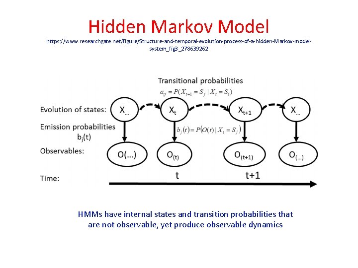
Hidden Markov Model https: //www. researchgate. net/figure/Structure-and-temporal-evolution-process-of-a-hidden-Markov-modelsystem_fig 3_278639262 HMMs have internal states and transition probabilities that are not observable, yet produce observable dynamics

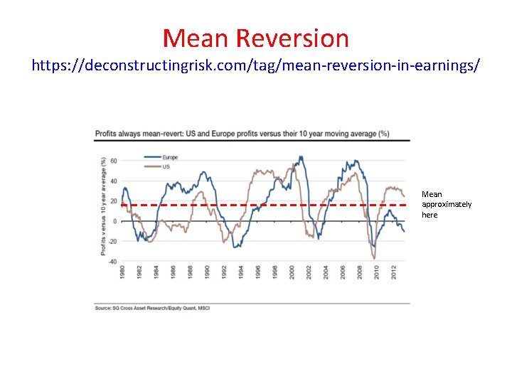
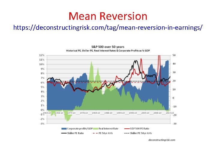
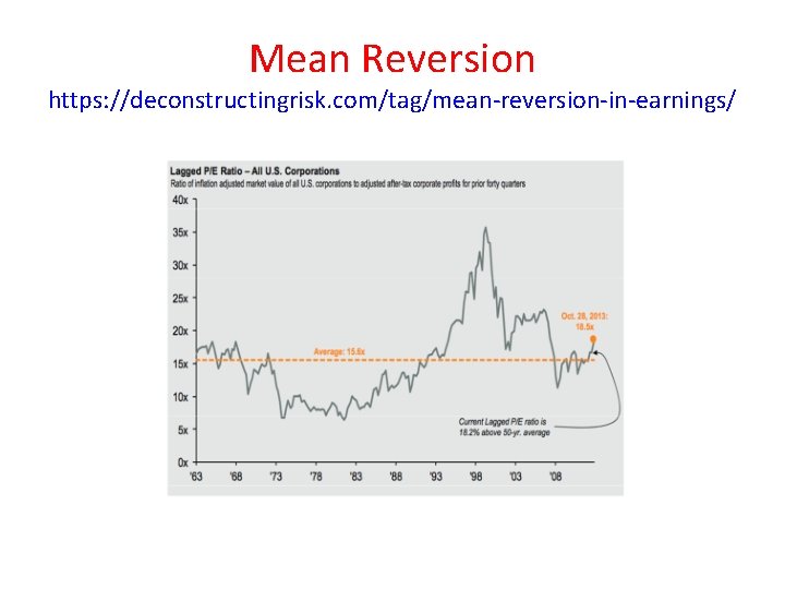
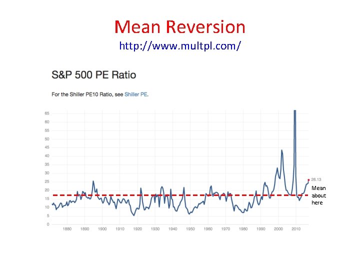
Mean Reversion https: //en. wikipedia. org/wiki/Mean_reversion_(finance) • In finance, mean reversion is the assumption that a stock's price will tend to move to the average price over time. • Using mean reversion in stock price analysis involves both identifying the trading range for a stock and computing the average price using analytical techniques taking into account considerations such as earnings, etc. • When the current market price is less than the average price, the stock is considered attractive for purchase, with the expectation that the price will rise (“value investing” or “oversold condition”). • When the current market price is above the average price, the market price is expected to fall (“momentum investing” or “overbought condition”) • In other words, deviations from the average price are expected to revert to the average. • Stock reporting services commonly offer moving averages for periods such as 50 and 100 days. • While reporting services provide the averages, identifying the high and low prices for the study period is still necessary.

Mean Reversion https: //deconstructingrisk. com/tag/mean-reversion-in-earnings/ Mean approximately here

Mean Reversion https: //deconstructingrisk. com/tag/mean-reversion-in-earnings/

Mean Reversion https: //deconstructingrisk. com/tag/mean-reversion-in-earnings/

Mean Reversion http: //www. multpl. com/ Mean about here

Time Series Prediction https: //en. wikipedia. org/wiki/Time_series • In statistics, prediction is a part of statistical inference. • One particular approach to such inference is known as predictive inference, but the prediction can be undertaken within any of the several approaches to statistical inference. • Indeed, one description of statistics is that it provides a means of transferring knowledge about a sample of a population to the whole population, and to other related populations, which is not necessarily the same as prediction over time. • An example of this is out-of-sample prediction and/or testing • When information is transferred across time, often to specific points in time, the process is known as forecasting. • When information describes only the current state, it is called nowcasting.

Time Series Prediction https: //en. wikipedia. org/wiki/Time_series • Stochastic simulation is used to generate alternative versions of the time series, representing what might happen over non-specific time-periods in the future • Conditional prediction is also based on statistical models to describe the likely outcome of the time series in the immediate future, given knowledge of the most recent outcomes (forecasting). • An example of this type of conditional prediction is often based on Bayes theorem • Forecasting on time series is usually done using automated statistical software packages and programming languages, such as R, S, SAS, SPSS, Minitab, pandas (Python) and many others.

Time Series Analysis Tools https: //en. wikipedia. org/wiki/Time_series Tools for investigating time-series data include: • Consideration of the autocorrelation function and the spectral density function (also cross-correlation functions and cross-spectral density functions) • Scaled or filtered cross- and auto-correlation functions to remove contributions of slow components • Performing a Fourier transform to investigate the series in the frequency domain • Use of a filter to remove unwanted noise or frequency components • Principal component analysis (or empirical orthogonal function analysis) • Singular spectrum analysis

Time Series Analysis Tools https: //en. wikipedia. org/wiki/Time_series Tools for investigating time-series data include: • • • Machine Learning Artificial neural networks Support Vector Machine Fuzzy Logic Gaussian Processes Hidden Markov model Queueing Theory Analysis Control chart Cumulative Sum (CUSUM) chart Exponentially Weighted Moving Average (EWMA) chart

Time Series Analysis Tools https: //en. wikipedia. org/wiki/Time_series Tools for investigating time-series data include: • • • Detrended fluctuation analysis Dynamic time warping Cross-correlation Dynamic Bayesian network Time-frequency analysis techniques: o Fast Fourier Transform o Continuous wavelet transform o Short-time Fourier transform o Chirplet transform o Fractional Fourier transform

Time Series Analysis Tools https: //en. wikipedia. org/wiki/Time_series Tools for investigating time-series data include: • Chaotic analysis o o o Correlation dimension Recurrence plots Recurrence quantification analysis Lyapunov exponents Entropy encoding

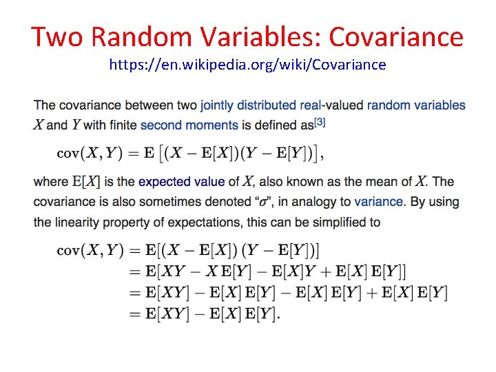
Two Random Variables: Covariance https: //en. wikipedia. org/wiki/Covariance • Recall that covariance is a measure of the joint variability of two random variables. • If the greater values of one variable mainly correspond with the greater values of the other variable, and the same holds for the lesser values, i. e. , the variables tend to show similar behavior, the covariance is positive. • In the opposite case, when the greater values of one variable mainly correspond to the lesser values of the other, i. e. , the variables tend to show opposite behavior, the covariance is negative

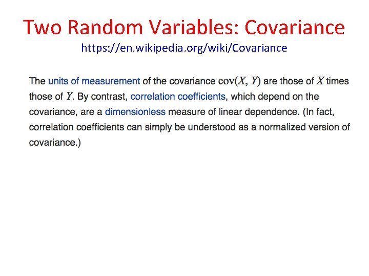
Two Random Variables: Covariance https: //en. wikipedia. org/wiki/Covariance Mental Picture: • • • As a balloon is blown up it gets larger in all dimensions, indicating positive covariance. If a sealed balloon is squashed in one dimension then it will expand in the other two, indicating negative covariance. The sign of the covariance therefore shows the tendency in the linear relationship between the variables. The magnitude of the covariance is not easy to interpret. The normalized version of the covariance, the correlation coefficient, however, shows by its magnitude the strength of the linear relation.

Two Random Variables: Covariance https: //en. wikipedia. org/wiki/Covariance

Two Random Variables: Covariance https: //en. wikipedia. org/wiki/Covariance

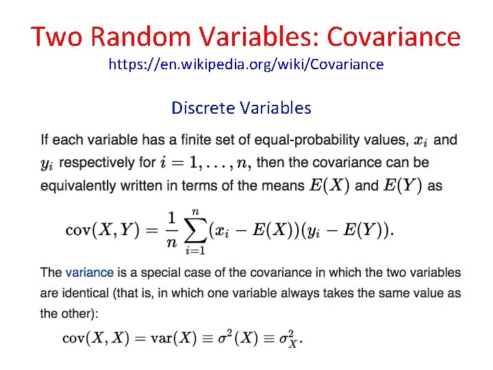
Two Random Variables: Covariance https: //en. wikipedia. org/wiki/Covariance Discrete Variables

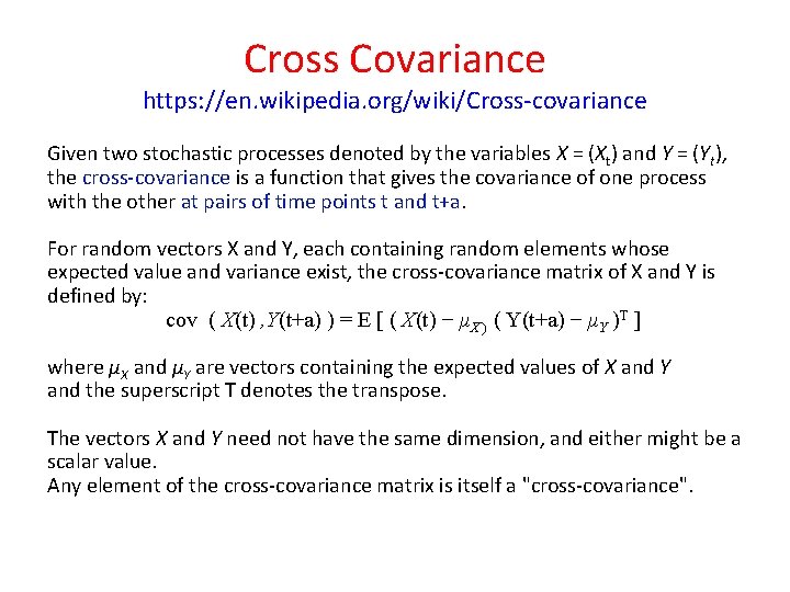
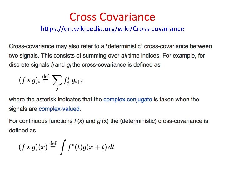
Cross Covariance https: //en. wikipedia. org/wiki/Cross-covariance Given two stochastic processes denoted by the variables X = (Xt) and Y = (Yt), the cross-covariance is a function that gives the covariance of one process with the other at pairs of time points t and t+a. For random vectors X and Y, each containing random elements whose expected value and variance exist, the cross-covariance matrix of X and Y is defined by: cov ( X(t) , Y(t+a) ) = E [ ( X(t) − μX ) ( Y(t+a) − μY )T ] where μX and μY are vectors containing the expected values of X and Y and the superscript T denotes the transpose. The vectors X and Y need not have the same dimension, and either might be a scalar value. Any element of the cross-covariance matrix is itself a "cross-covariance".

Cross Covariance https: //en. wikipedia. org/wiki/Cross-covariance

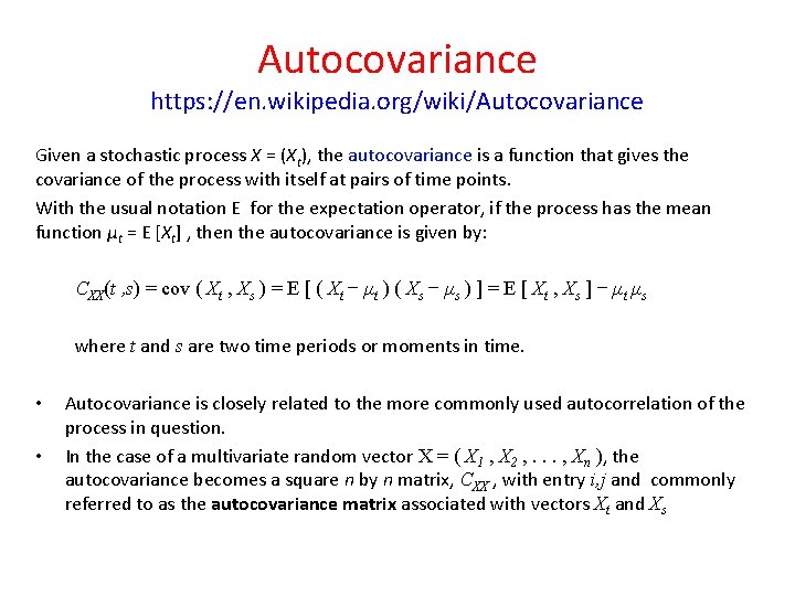
Autocovariance https: //en. wikipedia. org/wiki/Autocovariance Given a stochastic process X = (Xt), the autocovariance is a function that gives the covariance of the process with itself at pairs of time points. With the usual notation E for the expectation operator, if the process has the mean function μt = E [Xt] , then the autocovariance is given by: CXX(t , s) = cov ( Xt , Xs ) = E [ ( Xt − μt ) ( Xs − μs ) ] = E [ Xt , Xs ] − μt μs • • where t and s are two time periods or moments in time. Autocovariance is closely related to the more commonly used autocorrelation of the process in question. In the case of a multivariate random vector X = ( X 1 , X 2 , . . . , Xn ), the autocovariance becomes a square n by n matrix, CXX , with entry i, j and commonly referred to as the autocovariance matrix associated with vectors Xt and Xs

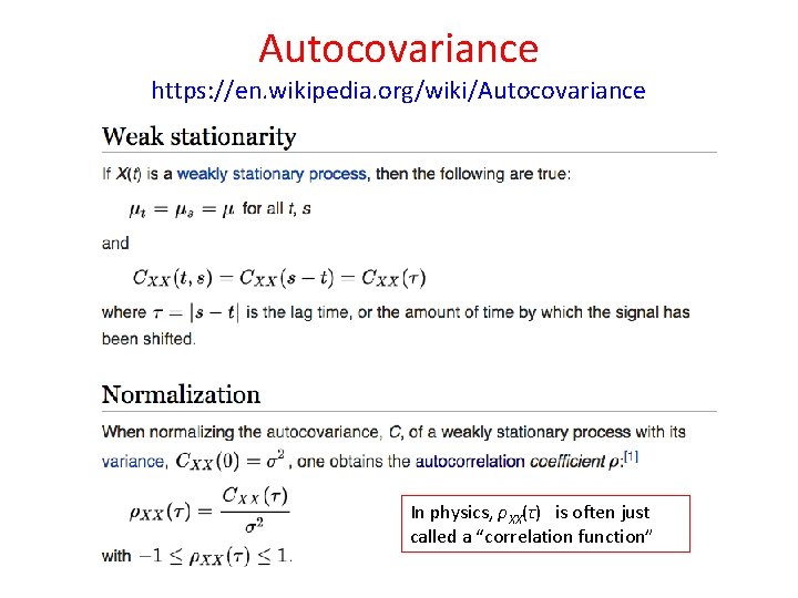
Autocovariance https: //en. wikipedia. org/wiki/Autocovariance In physics, ρXX(τ) is often just called a “correlation function”

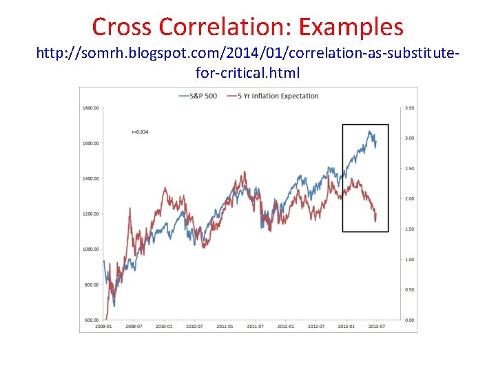
Cross Correlation: Examples http: //somrh. blogspot. com/2014/01/correlation-as-substitutefor-critical. html

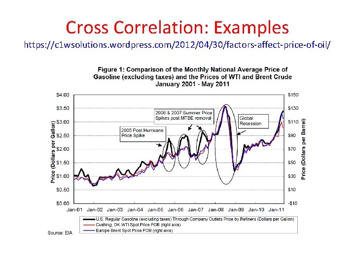
Cross Correlation: Examples https: //c 1 wsolutions. wordpress. com/2012/04/30/factors-affect-price-of-oil/

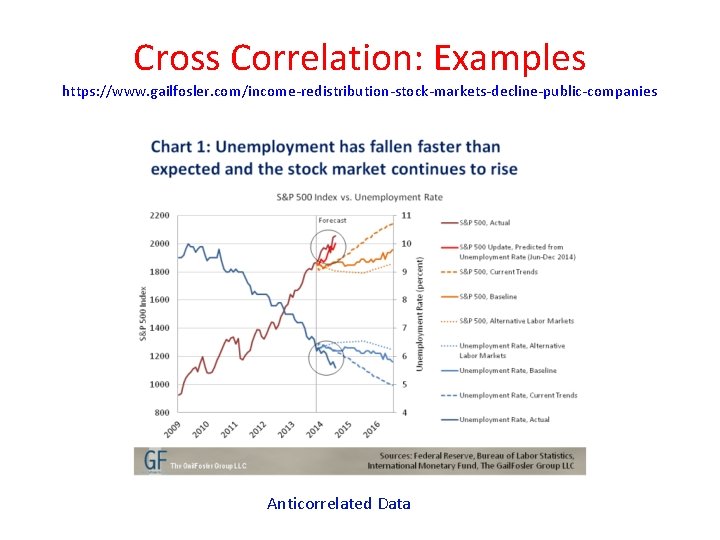
Cross Correlation: Examples https: //www. gailfosler. com/income-redistribution-stock-markets-decline-public-companies Anticorrelated Data

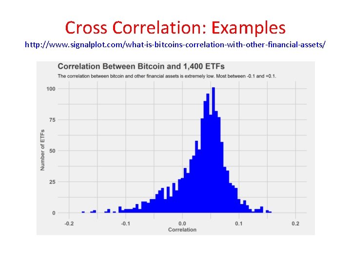
Cross Correlation: Examples http: //www. signalplot. com/what-is-bitcoins-correlation-with-other-financial-assets/

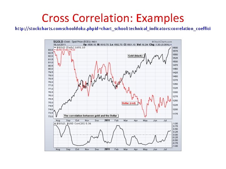
Cross Correlation: Examples http: //stockcharts. comschooldoku. phpid=chart_school: technical_indicators: correlation_coeffici

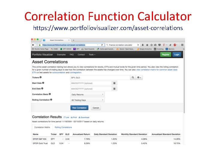
Correlation Function Calculator https: //www. portfoliovisualizer. com/asset-correlations

Correlation Functions https: //en. wikipedia. org/wiki/Correlation_function • With these definitions, the study of correlation functions is similar to the study of probability distributions. • Many stochastic processes can be completely characterized by their correlation functions • The most notable example is the class of Gaussian processes. • Probability distributions defined on a finite number of points can always be normalized, but when these are defined over continuous spaces, then extra care is called for. • The study of such distributions started with the study of random walks and led to the notion of the Itō calculus. • The Feynman path integral in Euclidean space generalizes this to other problems of interest to statistical mechanics.

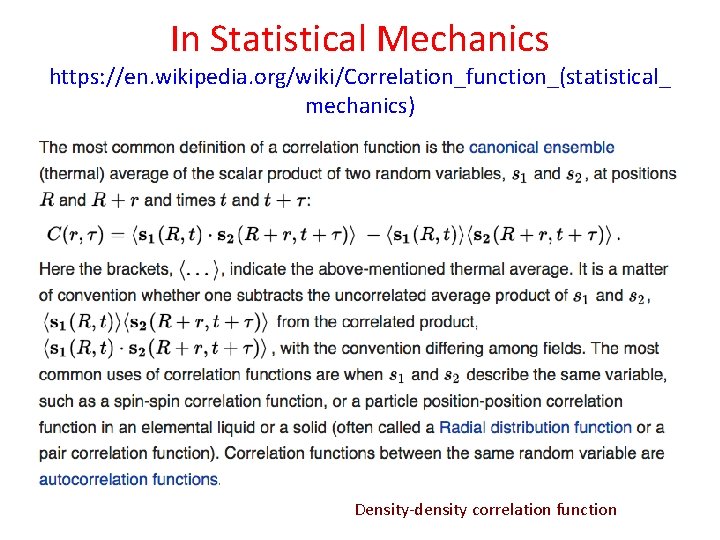
In Statistical Mechanics https: //en. wikipedia. org/wiki/Correlation_function_(statistical_ mechanics) Density-density correlation function

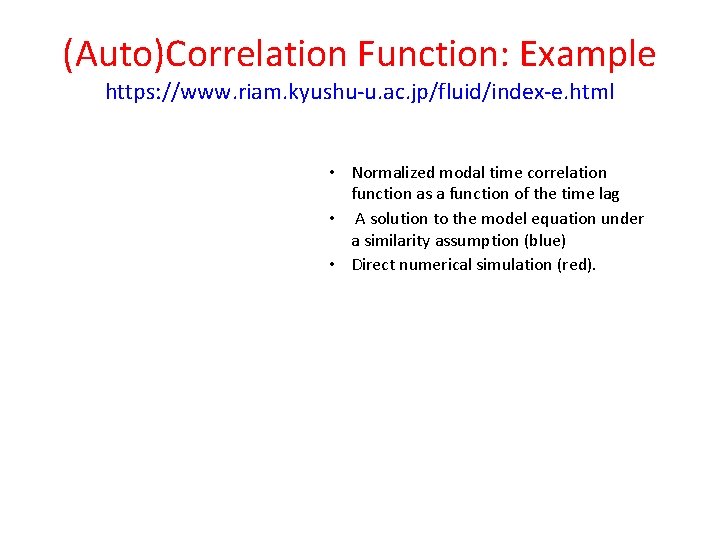
(Auto)Correlation Function: Example https: //www. riam. kyushu-u. ac. jp/fluid/index-e. html • Normalized modal time correlation function as a function of the time lag • A solution to the model equation under a similarity assumption (blue) • Direct numerical simulation (red).

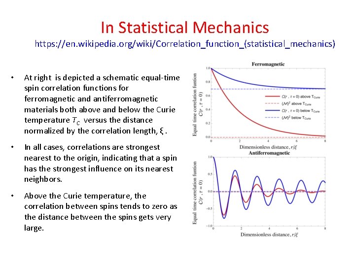
In Statistical Mechanics https: //en. wikipedia. org/wiki/Correlation_function_(statistical_mechanics) • At right is depicted a schematic equal-time spin correlation functions for ferromagnetic and antiferromagnetic materials both above and below the Curie temperature TC versus the distance normalized by the correlation length, ξ. • In all cases, correlations are strongest nearest to the origin, indicating that a spin has the strongest influence on its nearest neighbors. • Above the Curie temperature, the correlation between spins tends to zero as the distance between the spins gets very large.

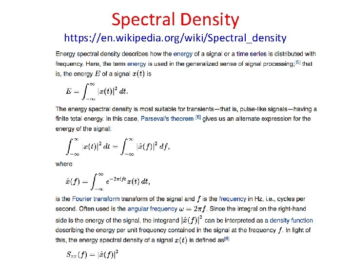
Spectral Density https: //en. wikipedia. org/wiki/Spectral_density

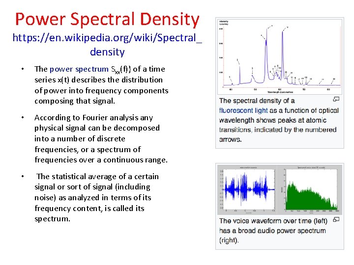
Power Spectral Density https: //en. wikipedia. org/wiki/Spectral_ density • The power spectrum Sxx(f)} of a time series x(t) describes the distribution of power into frequency components composing that signal. • According to Fourier analysis any physical signal can be decomposed into a number of discrete frequencies, or a spectrum of frequencies over a continuous range. • The statistical average of a certain signal or sort of signal (including noise) as analyzed in terms of its frequency content, is called its spectrum.

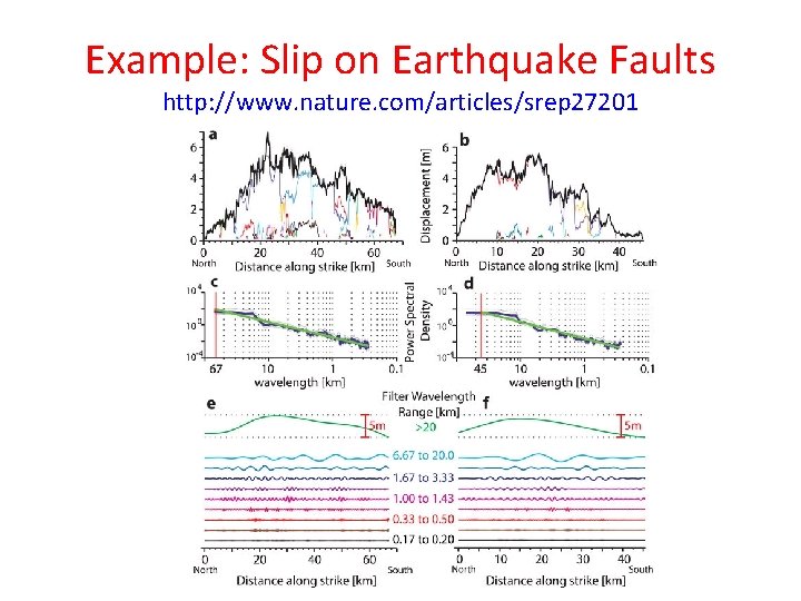
Example: Slip on Earthquake Faults http: //www. nature. com/articles/srep 27201

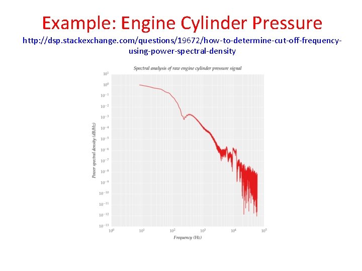
Example: Engine Cylinder Pressure http: //dsp. stackexchange. com/questions/19672/how-to-determine-cut-off-frequencyusing-power-spectral-density

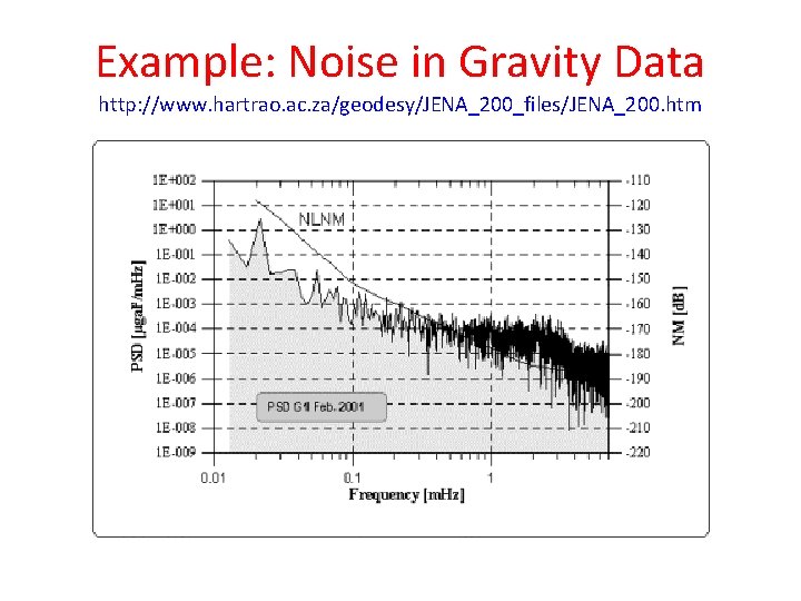
Example: Noise in Gravity Data http: //www. hartrao. ac. za/geodesy/JENA_200_files/JENA_200. htm

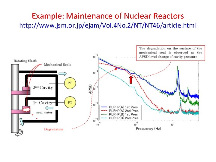
Example: Maintenance of Nuclear Reactors http: //www. jsm. or. jp/ejam/Vol. 4 No. 2/NT/NT 46/article. html

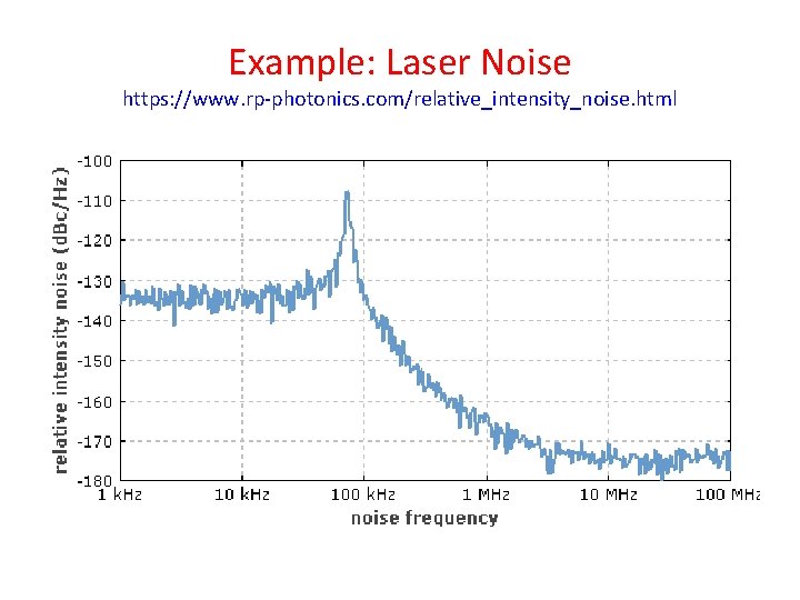
Example: Laser Noise https: //www. rp-photonics. com/relative_intensity_noise. html

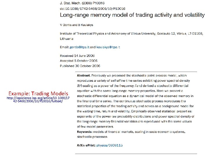
Example: Trading Models http: //iopscience. iop. org/article/10. 1088/17 42 -5468/2006/10/P 10016/fulltext/

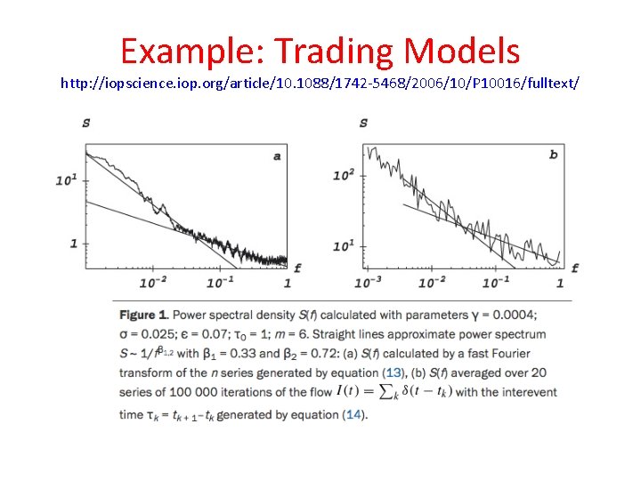
Example: Trading Models http: //iopscience. iop. org/article/10. 1088/1742 -5468/2006/10/P 10016/fulltext/

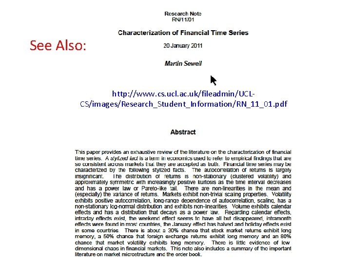
See Also: http: //www. cs. ucl. ac. uk/fileadmin/UCLCS/images/Research_Student_Information/RN_11_01. pdf

See Also: http: //www. lmd. ens. fr/E 2 C 2/class/SASP_lecture_notes. pdf