Lecture 13 Diagnostics in MLR Variance Inflation Factors

Lecture 13 Diagnostics in MLR Variance Inflation Factors Added variable plots Identifying outliers BMTRY 701 Biostatistical Methods II

Variance Inflation Factor (VIF) § Diagnostic for multicollinearity § Describes the amount of an X that is explained by the other X’s in the model § If VIF is high, then it suggests that the covariate should not be added. § Why? • it is redundant • it adds variance to the model • it creates ‘instability’ in the estimation

How to calculate VIF? § Simple idea: § That is, the VIF for the jth covariate is the coefficient of determination (R 2) obtained from regressing xj on the remaining x’s in the model

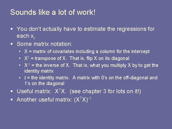
Sounds like a lot of work! § You don’t actually have to estimate the regressions for each xj. § Some matrix notation: • X = matrix of covariates including a column for the intercept • XT = transpose of X. That is, flip X on its diagonal • X-1 = the inverse of X. That is, what you multiply X by to get the identity matrix • I = the identity matrix. A matrix with 0’s on the off-diagonal and 1’s on the diagonal § Useful matrix: XTX. (see chapter 3 for lots on it!) § Another useful matrix: (XTX)-1

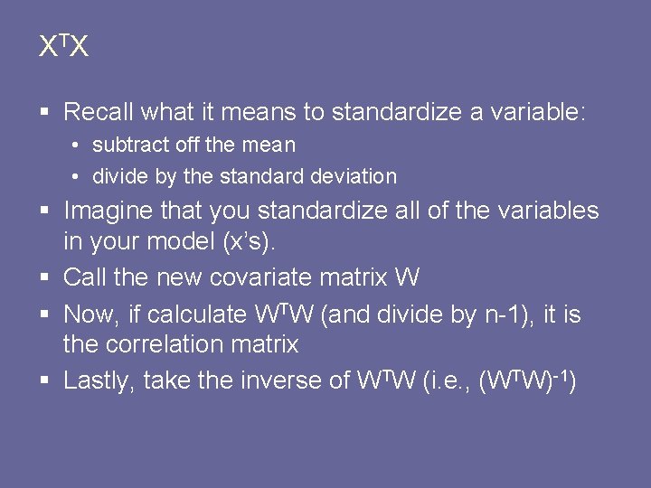
X TX § Recall what it means to standardize a variable: • subtract off the mean • divide by the standard deviation § Imagine that you standardize all of the variables in your model (x’s). § Call the new covariate matrix W § Now, if calculate WTW (and divide by n-1), it is the correlation matrix § Lastly, take the inverse of WTW (i. e. , (WTW)-1)

VIFs § The diagonals of the (WTW)-1 matrix are the VIFs § This is a natural by-product of the regression § The (WTW)-1 matrix is estimated when the regression is estimated § Rules of thumb: • VIF larger than 10 implies a serious multicollinearity problem • VIFs of 5 or greater suggest that coefficient estimates may be misleading due to multicollinearity

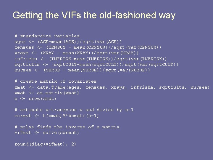
Getting the VIFs the old-fashioned way # standardize variables ages <- (AGE-mean(AGE))/sqrt(var(AGE)) censuss <- (CENSUS - mean(CENSUS))/sqrt(var(CENSUS)) xrays <- (XRAY - mean(XRAY))/sqrt(var(XRAY)) infrisks <- (INFRISK-mean(INFRISK))/sqrt(var(INFRISK)) sqrtcults <- (sqrt. CULT-mean(sqrt. CULT))/sqrt(var(sqrt. CULT)) nurses <- (NURSE - mean(NURSE))/sqrt(var(NURSE)) # create matrix of covariates xmat <- data. frame(ages, censuss, xrays, infrisks, sqrtcults, nurses) xmat <- as. matrix(xmat) n <- nrow(xmat) # estimate x-transpose x and divide by n-1 cormat <- t(xmat)%*%xmat/(n-1) # solve finds the inverse of a matrix vifmat <- solve(cormat) round(diag(vifmat), 2)

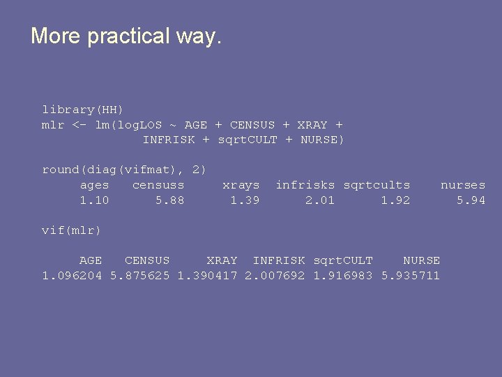
More practical way. library(HH) mlr <- lm(log. LOS ~ AGE + CENSUS + XRAY + INFRISK + sqrt. CULT + NURSE) round(diag(vifmat), 2) ages censuss 1. 10 5. 88 xrays 1. 39 infrisks sqrtcults 2. 01 1. 92 vif(mlr) nurses 5. 94 AGE CENSUS XRAY INFRISK sqrt. CULT NURSE 1. 096204 5. 875625 1. 390417 2. 007692 1. 916983 5. 935711

What to do? § Unlikely that only one variable will have high VIF § You need to then determine which to include, which to remove § Judgement should be based on science + statistics!

More diagnostics: the added variable plots § These can help check for adequacy of model § Is there curvature between Y and X after adjusting for the other X’s? § “Refined” residual plots § They show the marginal importance of an individual predictor § Help figure out a good form for the predictor

Example: SENIC § Recall the difficulty determining the form for INFIRSK in our regression model. § Last time, we settled on including one term, INFRISK^2 § But, we could do an adjusted variable plot approach. § How? § We want to know, adjusting for all else in the model, what is the right form for INFRISK?

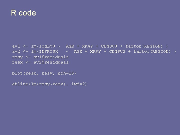
R code av 1 <- lm(log. LOS ~ AGE + XRAY + CENSUS + factor(REGION) ) av 2 <- lm(INFRISK ~ AGE + XRAY + CENSUS + factor(REGION) ) resy <- av 1$residuals resx <- av 2$residuals plot(resx, resy, pch=16) abline(lm(resy~resx), lwd=2)

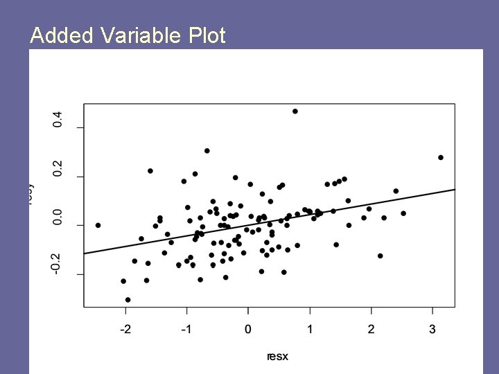
Added Variable Plot

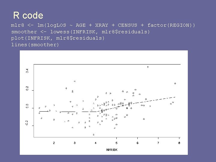
What does that show? § The relationship between log. LOS and INFRISK if you added INFRISK to the regression § But, is that we want to see? § How about looking at residuals versus INFRISK (before including INFRISK in the model)?

R code mlr 8 <- lm(log. LOS ~ AGE + XRAY + CENSUS + factor(REGION)) smoother <- lowess(INFRISK, mlr 8$residuals) plot(INFRISK, mlr 8$residuals) lines(smoother)

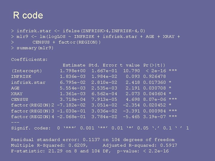
R code > infrisk. star <- ifelse(INFRISK>4, INFRISK-4, 0) > mlr 9 <- lm(log. LOS ~ INFRISK + infrisk. star + AGE + XRAY + > CENSUS + factor(REGION)) > summary(mlr 9) Coefficients: Estimate Std. Error t value Pr(>|t|) (Intercept) 1. 798 e+00 1. 667 e-01 10. 790 < 2 e-16 *** INFRISK 1. 836 e-03 1. 984 e-02 0. 093 0. 926478 infrisk. star 6. 795 e-02 2. 810 e-02 2. 418 0. 017360 * AGE 5. 554 e-03 2. 535 e-03 2. 191 0. 030708 * XRAY 1. 361 e-03 6. 562 e-04 2. 073 0. 040604 * CENSUS 3. 718 e-04 7. 913 e-05 4. 698 8. 07 e-06 *** factor(REGION)2 -7. 182 e-02 3. 051 e-02 -2. 354 0. 020452 * factor(REGION)3 -1. 030 e-01 3. 036 e-02 -3. 391 0. 000984 *** factor(REGION)4 -2. 068 e-01 3. 784 e-02 -5. 465 3. 19 e-07 *** --Signif. codes: 0 ‘***’ 0. 001 ‘**’ 0. 01 ‘*’ 0. 05 ‘. ’ 0. 1 ‘ ’ 1 Residual standard error: 0. 1137 on 104 degrees of freedom Multiple R-Squared: 0. 6209, Adjusted R-squared: 0. 5917 F-statistic: 21. 29 on 8 and 104 DF, p-value: < 2. 2 e-16

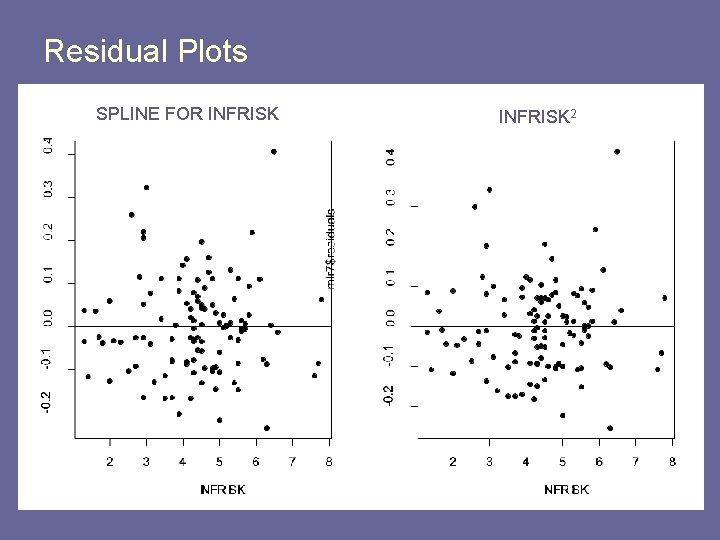
Residual Plots SPLINE FOR INFRISK 2

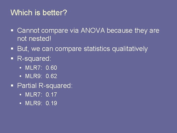
Which is better? § Cannot compare via ANOVA because they are not nested! § But, we can compare statistics qualitatively § R-squared: • MLR 7: 0. 60 • MLR 9: 0. 62 § Partial R-squared: • MLR 7: 0. 17 • MLR 9: 0. 19

Identifying Outliers § Harder to do in the MLR setting than in the SLR setting. § Recall two concepts that make outliers important: • Leverage is a function of the explanatory variable(s) alone and measures the potential for a data point to affect the model parameter estimates. • Influence is a measure of how much a data point actually does affect the estimated model. § Leverage and influence both may be defined in terms of matrices

“Hat” matrix § We must do some matrix stuff to understand this § Notation for a MLR with p predictors and data on n patients. § The data:

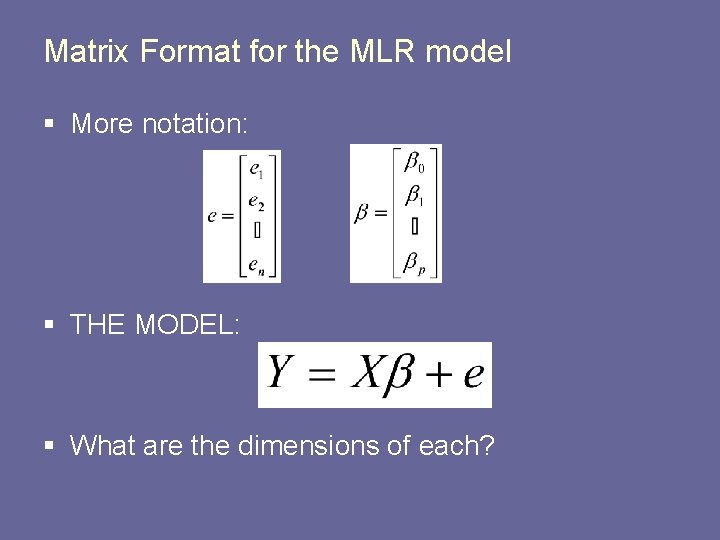
Matrix Format for the MLR model § More notation: § THE MODEL: § What are the dimensions of each?

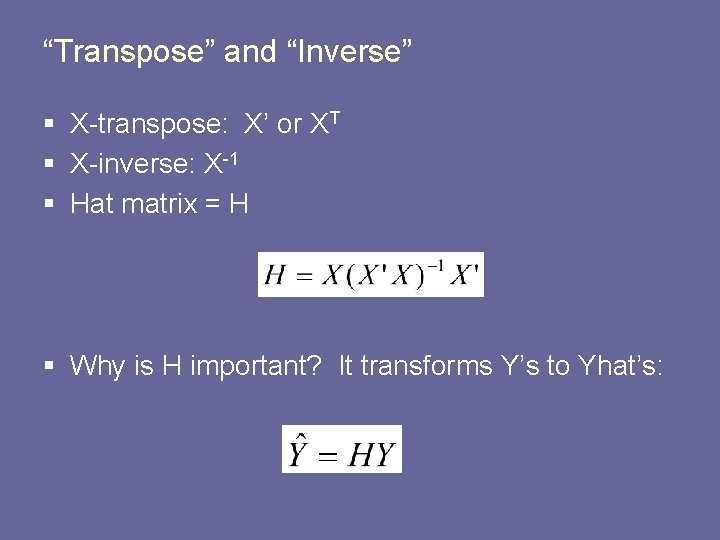
“Transpose” and “Inverse” § X-transpose: X’ or XT § X-inverse: X-1 § Hat matrix = H § Why is H important? It transforms Y’s to Yhat’s:

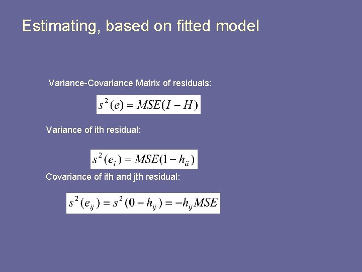
Estimating, based on fitted model Variance-Covariance Matrix of residuals: Variance of ith residual: Covariance of ith and jth residual:

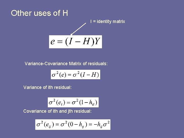
Other uses of H I = identity matrix Variance-Covariance Matrix of residuals: Variance of ith residual: Covariance of ith and jth residual:

Property of hij’s This means that each row of H sums to 1 And, that each column of H sums to 1

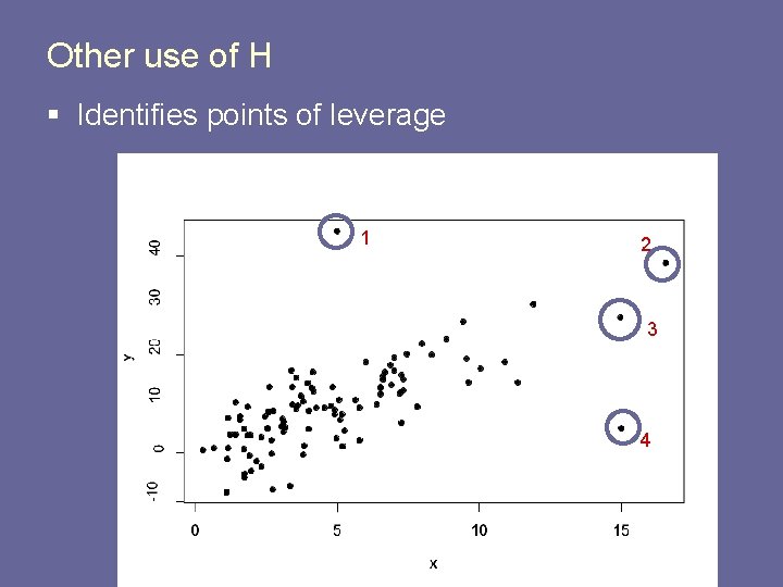
Other use of H § Identifies points of leverage 1 2 3 4

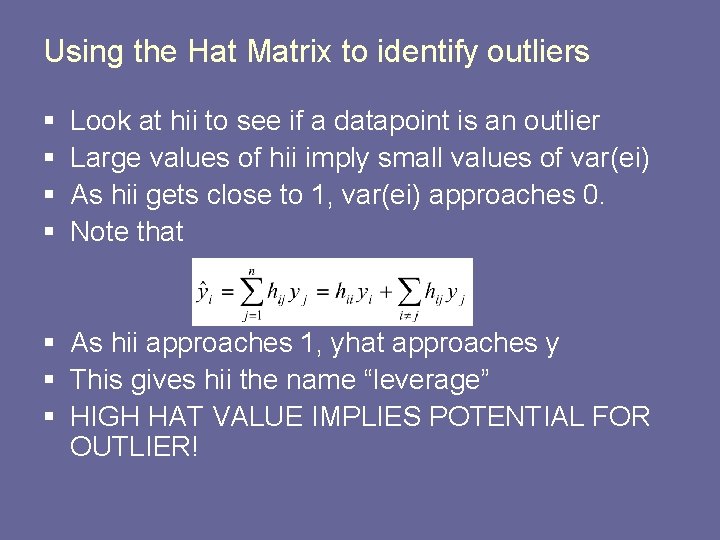
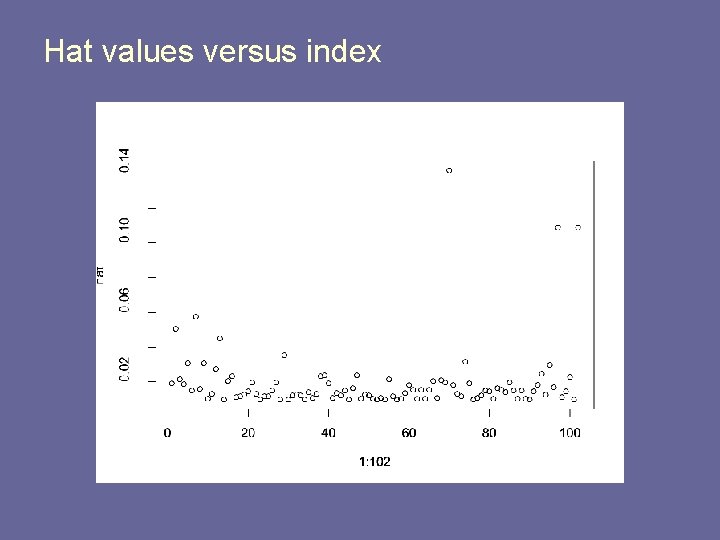
Using the Hat Matrix to identify outliers § § Look at hii to see if a datapoint is an outlier Large values of hii imply small values of var(ei) As hii gets close to 1, var(ei) approaches 0. Note that § As hii approaches 1, yhat approaches y § This gives hii the name “leverage” § HIGH HAT VALUE IMPLIES POTENTIAL FOR OUTLIER!

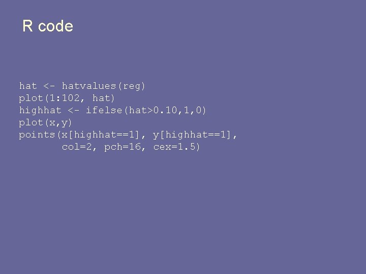
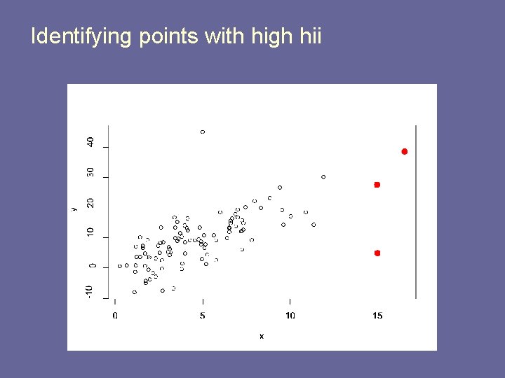
R code hat <- hatvalues(reg) plot(1: 102, hat) highhat <- ifelse(hat>0. 10, 1, 0) plot(x, y) points(x[highhat==1], y[highhat==1], col=2, pch=16, cex=1. 5)

Hat values versus index

Identifying points with high hii

Does a high hat mean it has a large residual? § No. § hii measures leverage, not influence § Recall what hii is made of • it depends ONLY on the X’s • it does not depend on the actual Y value § Look back at the plot: which of these is probably most “influential” § Standard cutoffs for “large” hii: • 2 p/n • 0. 5 very high, 0. 2 -0. 5 high

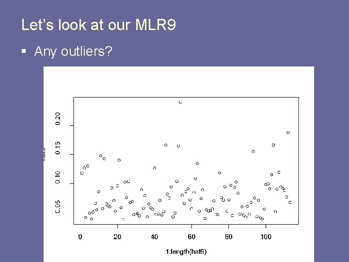
Let’s look at our MLR 9 § Any outliers?

Using the hat matrix in MLR § Studentized residuals § Acknowledge: • each residual has a different variance • magnitude of residual should be made relative to its variance (or sd) § Studentized residuals recognize differences in sampling errors

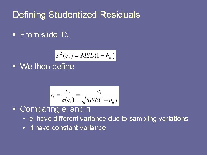
Defining Studentized Residuals § From slide 15, § We then define § Comparing ei and ri • ei have different variance due to sampling variations • ri have constant variance

Deleted Residuals § Influence is more intuitively quantified by how things change when an observation is in versus out of the estimation process § Would be more useful to have residuals in the situation when the observation is removed. § Example: • if a Yi is far out then it may be very influential in the regression and the residual will be small • but, if that case is removed before estimating and then the residual is calculated based on the fit, the residual would be large

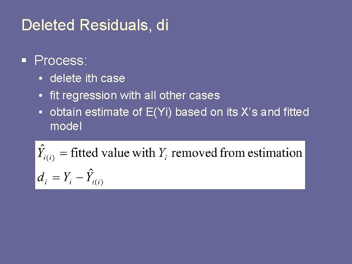
Deleted Residuals, di § Process: • delete ith case • fit regression with all other cases • obtain estimate of E(Yi) based on its X’s and fitted model

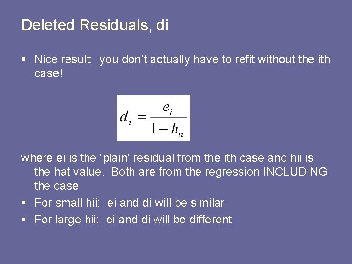
Deleted Residuals, di § Nice result: you don’t actually have to refit without the ith case! where ei is the ‘plain’ residual from the ith case and hii is the hat value. Both are from the regression INCLUDING the case § For small hii: ei and di will be similar § For large hii: ei and di will be different

Studentized Deleted Residuals § Recall the need to standardize, based on the knowledge of the variance § The difference between ti and ri?

Another nice result § You can calculate MSE(i) without refitting the model

Testing for outliers § outlier = Y observations whose studentized deleted residuals are large (in absolute value) § ti ~ t with n-p-1 degrees of freedom § Two examples: • simulated data • mlr 9