Lecture 13 Algorithm Analysis Arne Kutzner Hanyang University

Lecture 13 Algorithm Analysis Arne Kutzner Hanyang University / Seoul Korea

Single Source Shortest Paths

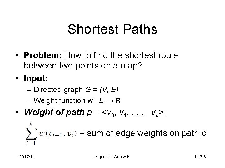
Shortest Paths • Problem: How to find the shortest route between two points on a map? • Input: – Directed graph G = (V, E) – Weight function w : E → R • Weight of path p = <v 0, v 1, . . . , vk> : = sum of edge weights on path p 2017/11 Algorithm Analysis L 13. 3

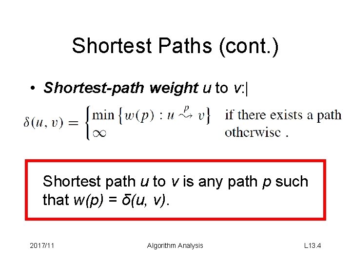
Shortest Paths (cont. ) • Shortest-path weight u to v: | Shortest path u to v is any path p such that w(p) = δ(u, v). 2017/11 Algorithm Analysis L 13. 4

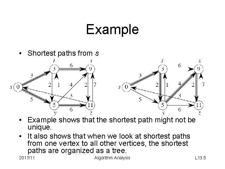
Example • Shortest paths from s • Example shows that the shortest path might not be unique. • It also shows that when we look at shortest paths from one vertex to all other vertices, the shortest paths are organized as a tree. 2017/11 Algorithm Analysis L 13. 5

Variants of Shortest Path Problem • Single-source: Find shortest paths from a given source vertex s ∈ V to every vertex v ∈ V. • Single-destination: Find shortest paths to a given destination vertex. • Single-pair: Find shortest path from u to v. No way known that’s better in worst case than solving single-source. • All-pairs: Find shortest path from u to v for all u, v ∈ V. 2017/11 Algorithm Analysis L 13. 6

Negative-Weight Edges • OK if the negative-weight cycle is not reachable from the source • If we have a negative-weight cycle, we can just keep going around it, and get w(s, v) = −∞ for all v on the cycle • Some algorithms work only if there are no negative-weight edges in the graph. 2017/11 Algorithm Analysis L 13. 7

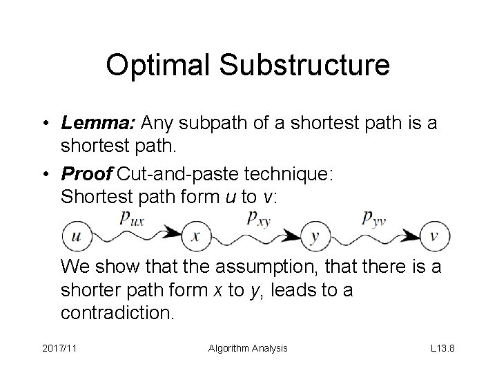
Optimal Substructure • Lemma: Any subpath of a shortest path is a shortest path. • Proof Cut-and-paste technique: Shortest path form u to v: We show that the assumption, that there is a shorter path form x to y, leads to a contradiction. 2017/11 Algorithm Analysis L 13. 8

Cycles • Shortest paths can not contain cycles: – Already ruled out negative-weight cycles. – Positive-weight ⇒ we can get a shorter path by omitting the cycle. – Zero-weight: no reason to use them ⇒ assume that our solutions won’t use them. 2017/11 Algorithm Analysis L 13. 9

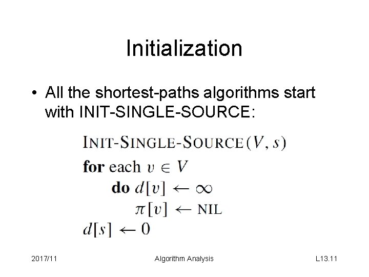
Output of Single-Source Shortest-Path Algorithm For each vertex v ∈ V: • d[v] = δ(s, v). – Initially, d[v]=∞. – Reduces as algorithms progress. But always maintain d[v] ≥ δ(s, v). – Call d[v] a shortest-path estimate. • π[v] = predecessor of v on a shortest path from s. – If no predecessor, π[v] = NIL. – π induces a tree. shortest-path tree. 2017/11 Algorithm Analysis L 13. 10

Initialization • All the shortest-paths algorithms start with INIT-SINGLE-SOURCE: 2017/11 Algorithm Analysis L 13. 11

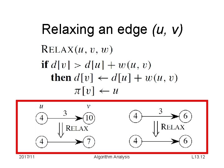
Relaxing an edge (u, v) 2017/11 Algorithm Analysis L 13. 12

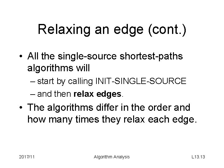
Relaxing an edge (cont. ) • All the single-source shortest-paths algorithms will – start by calling INIT-SINGLE-SOURCE – and then relax edges. • The algorithms differ in the order and how many times they relax each edge. 2017/11 Algorithm Analysis L 13. 13

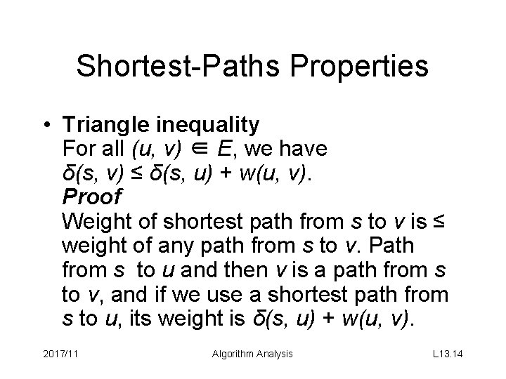
Shortest-Paths Properties • Triangle inequality For all (u, v) ∈ E, we have δ(s, v) ≤ δ(s, u) + w(u, v). Proof Weight of shortest path from s to v is ≤ weight of any path from s to v. Path from s to u and then v is a path from s to v, and if we use a shortest path from s to u, its weight is δ(s, u) + w(u, v). 2017/11 Algorithm Analysis L 13. 14

Shortest-Paths Properties (cont. ) • Upper-bound property (for Relaxing edges) We always have d[v] ≥ δ(s, v) for all v. Once d[v] = δ(s, v), it never changes. • No-path property (Corollary of Upper-bound prop. ) If δ(s, v)=∞, then always d[v]=∞ • Convergence property If the path from s to u and finally v is a shortest path, d[u] = δ(s, u), and we call RELAX(u, v, w), then d[v] = δ(s, v) afterward. • Path relaxation property Let p = <v 0, v 1, . . . , vk> be a shortest path from s = v 0 to vk. If we relax, in order, (v 0, v 1), (v 1, v 2), . . . , (vk− 1, vk), even intermixed with other relaxations, then d[vk ] = δ(s, vk ). 2017/11 Algorithm Analysis L 13. 15

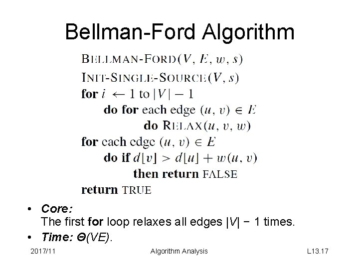
Bellman-Ford Algorithm • Allows negative-weight edges. • Computes d[v] and π[v] for all v ∈ V. • Returns TRUE if no negative-weight cycles reachable from s, FALSE otherwise 2017/11 Algorithm Analysis L 13. 16

Bellman-Ford Algorithm • Core: The first for loop relaxes all edges |V| − 1 times. • Time: Θ(VE). 2017/11 Algorithm Analysis L 13. 17

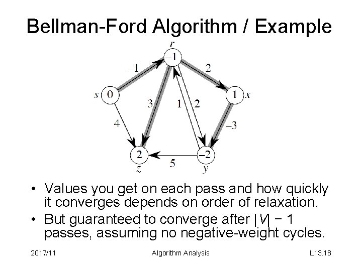
Bellman-Ford Algorithm / Example • Values you get on each pass and how quickly it converges depends on order of relaxation. • But guaranteed to converge after |V| − 1 passes, assuming no negative-weight cycles. 2017/11 Algorithm Analysis L 13. 18

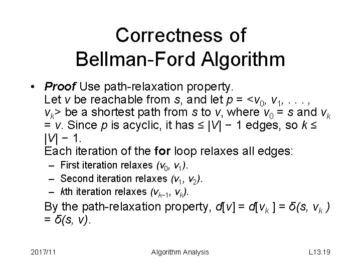
Correctness of Bellman-Ford Algorithm • Proof Use path-relaxation property. Let v be reachable from s, and let p = <v 0, v 1, . . . , vk> be a shortest path from s to v, where v 0 = s and vk = v. Since p is acyclic, it has ≤ |V| − 1 edges, so k ≤ |V| − 1. Each iteration of the for loop relaxes all edges: – First iteration relaxes (v 0, v 1). – Second iteration relaxes (v 1, v 2). – kth iteration relaxes (vk− 1, vk). By the path-relaxation property, d[v] = d[vk ] = δ(s, vk ) = δ(s, v). 2017/11 Algorithm Analysis L 13. 19

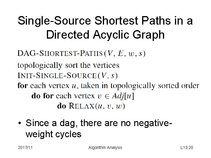
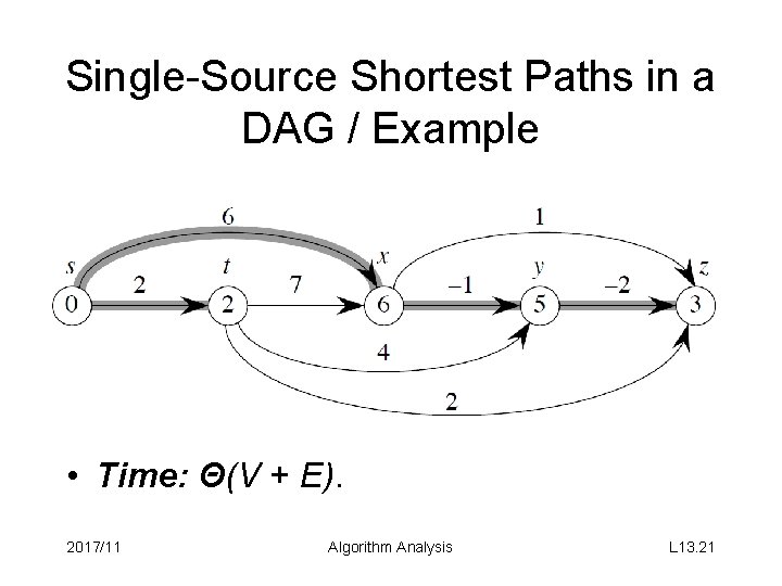
Single-Source Shortest Paths in a Directed Acyclic Graph • Since a dag, there are no negativeweight cycles 2017/11 Algorithm Analysis L 13. 20

Single-Source Shortest Paths in a DAG / Example • Time: Θ(V + E). 2017/11 Algorithm Analysis L 13. 21

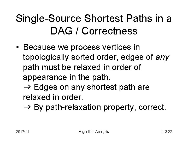
Single-Source Shortest Paths in a DAG / Correctness • Because we process vertices in topologically sorted order, edges of any path must be relaxed in order of appearance in the path. ⇒ Edges on any shortest path are relaxed in order. ⇒ By path-relaxation property, correct. 2017/11 Algorithm Analysis L 13. 22

Dijkstra’s Algorithm

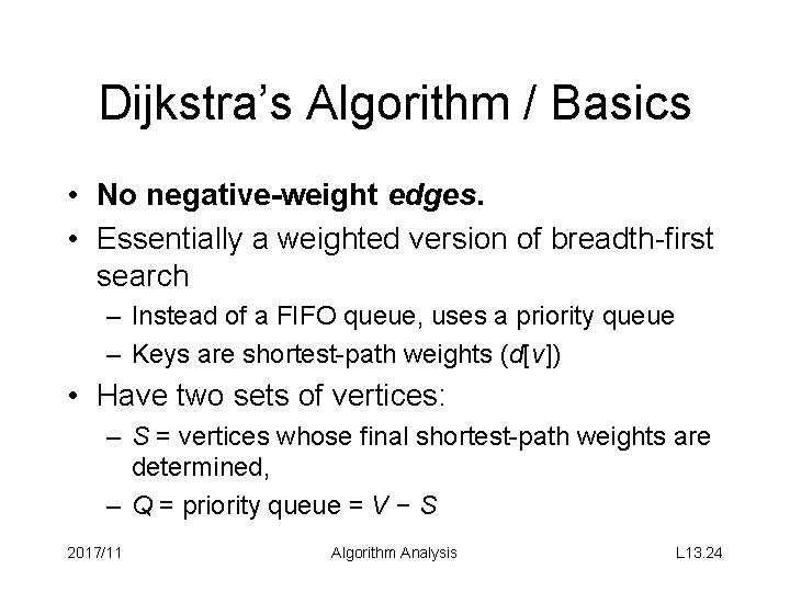
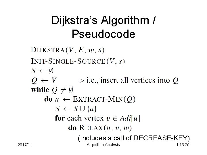
Dijkstra’s Algorithm / Basics • No negative-weight edges. • Essentially a weighted version of breadth-first search – Instead of a FIFO queue, uses a priority queue – Keys are shortest-path weights (d[v]) • Have two sets of vertices: – S = vertices whose final shortest-path weights are determined, – Q = priority queue = V − S 2017/11 Algorithm Analysis L 13. 24

Dijkstra’s Algorithm / Pseudocode (Includes a call of DECREASE-KEY) 2017/11 Algorithm Analysis L 13. 25

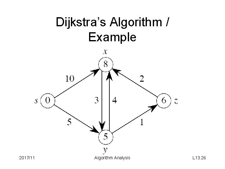
Dijkstra’s Algorithm / Example 2017/11 Algorithm Analysis L 13. 26

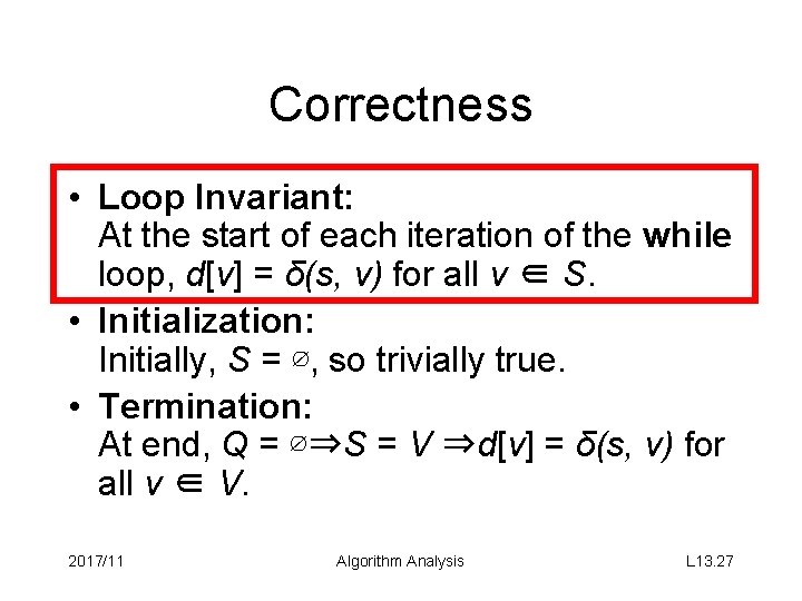
Correctness • Loop Invariant: At the start of each iteration of the while loop, d[v] = δ(s, v) for all v ∈ S. • Initialization: Initially, S = ∅, so trivially true. • Termination: At end, Q = ∅⇒S = V ⇒d[v] = δ(s, v) for all v ∈ V. 2017/11 Algorithm Analysis L 13. 27

Correctness / Maintenance (loop invariant) • Need to show that d[u] = δ(s, u) when u is added to S in each iteration. • Suppose there exists u such that d[u] ≠ δ(s, u). Without loss of generality, let u be the first vertex for which d[u] ≠ δ(s, u) when u is added to S. • Observations: • u ≠ s, since d[s] = δ(s, s) = 0. • Therefore, s ∈ S, so S ≠ ∅. • There must be some path from s to u, since otherwise d[u] = δ(s, u) = ∞ by no-path property. 2017/11 Algorithm Analysis L 13. 28

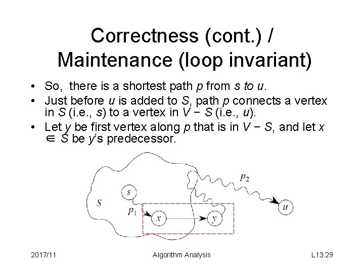
Correctness (cont. ) / Maintenance (loop invariant) • So, there is a shortest path p from s to u. • Just before u is added to S, path p connects a vertex in S (i. e. , s) to a vertex in V − S (i. e. , u). • Let y be first vertex along p that is in V − S, and let x ∈ S be y’s predecessor. 2017/11 Algorithm Analysis L 13. 29

Correctness (cont. ) / Maintenance (loop invariant) • Claim: d[y] = δ(s, y) when u is added to S. • Proof: x ∈ S and u is the first vertex such that d[u] ≠ δ(s, u) when u is added to S ⇒d[x] = δ(s, x) when x is added to S. Relaxed (x, y) at that time, so by the convergence property, d[y] = δ(s, y). 2017/11 Algorithm Analysis L 13. 30

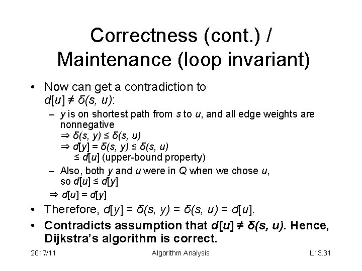
Correctness (cont. ) / Maintenance (loop invariant) • Now can get a contradiction to d[u] ≠ δ(s, u): – y is on shortest path from s to u, and all edge weights are nonnegative ⇒ δ(s, y) ≤ δ(s, u) ⇒ d[y] = δ(s, y) ≤ δ(s, u) ≤ d[u] (upper-bound property) – Also, both y and u were in Q when we chose u, so d[u] ≤ d[y] ⇒ d[u] = d[y] • Therefore, d[y] = δ(s, y) = δ(s, u) = d[u]. • Contradicts assumption that d[u] ≠ δ(s, u). Hence, Dijkstra’s algorithm is correct. 2017/11 Algorithm Analysis L 13. 31

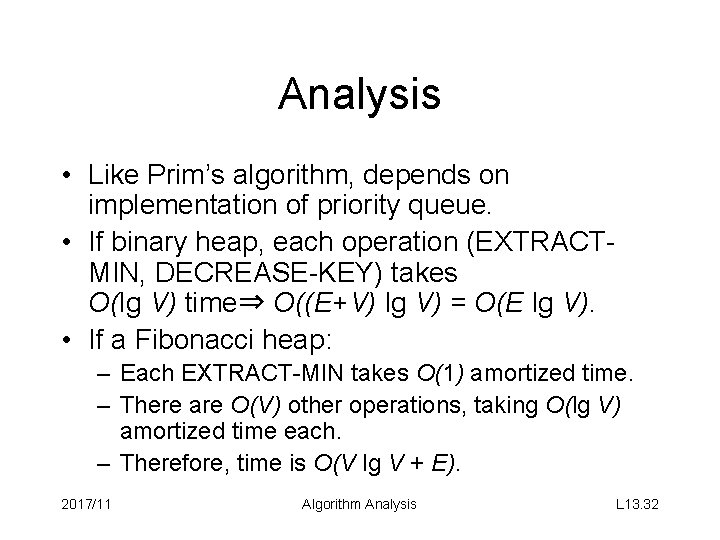
Analysis • Like Prim’s algorithm, depends on implementation of priority queue. • If binary heap, each operation (EXTRACTMIN, DECREASE-KEY) takes O(lg V) time⇒ O((E+V) lg V) = O(E lg V). • If a Fibonacci heap: – Each EXTRACT-MIN takes O(1) amortized time. – There are O(V) other operations, taking O(lg V) amortized time each. – Therefore, time is O(V lg V + E). 2017/11 Algorithm Analysis L 13. 32