Lecture 12 Object Detection and Recognition What is

第十二章目标检测与识别 Lecture 12 Object Detection and Recognition

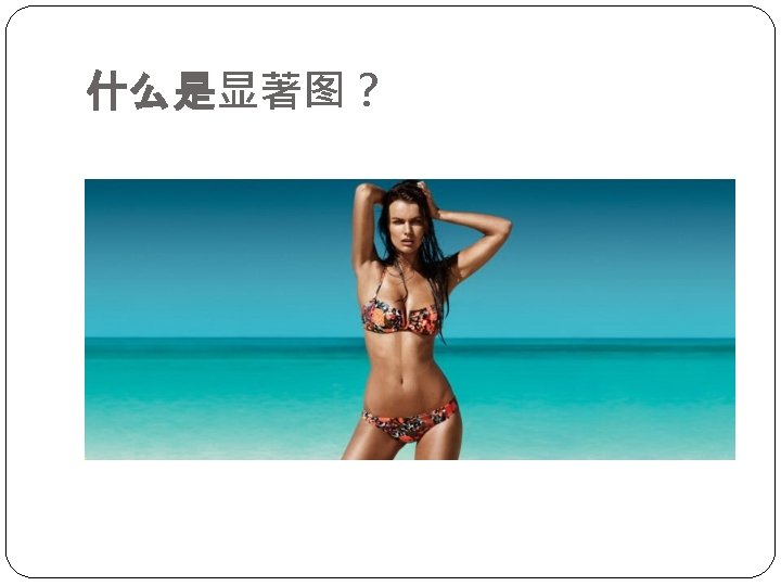
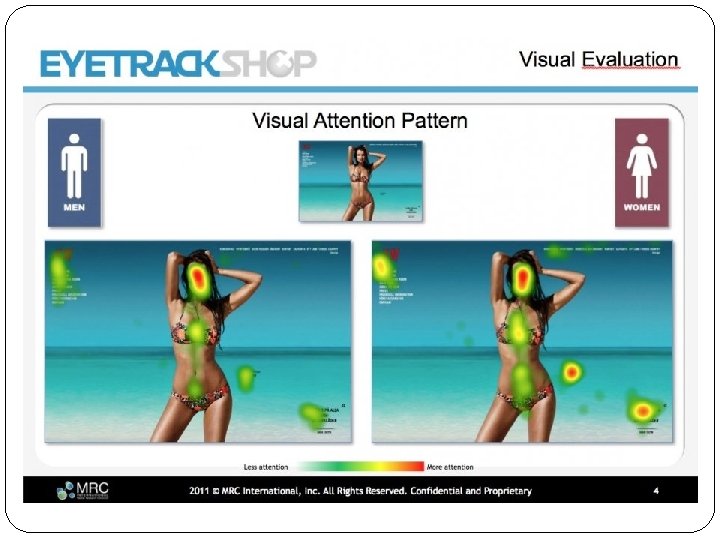
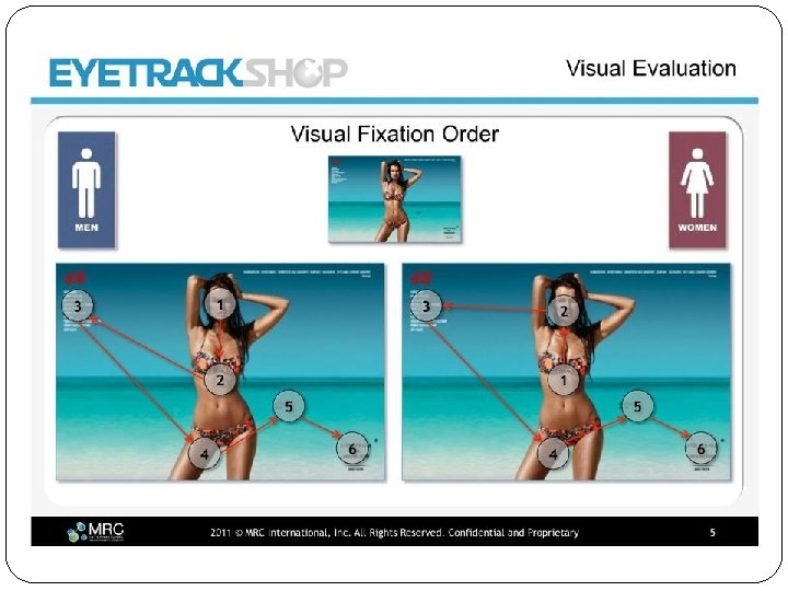
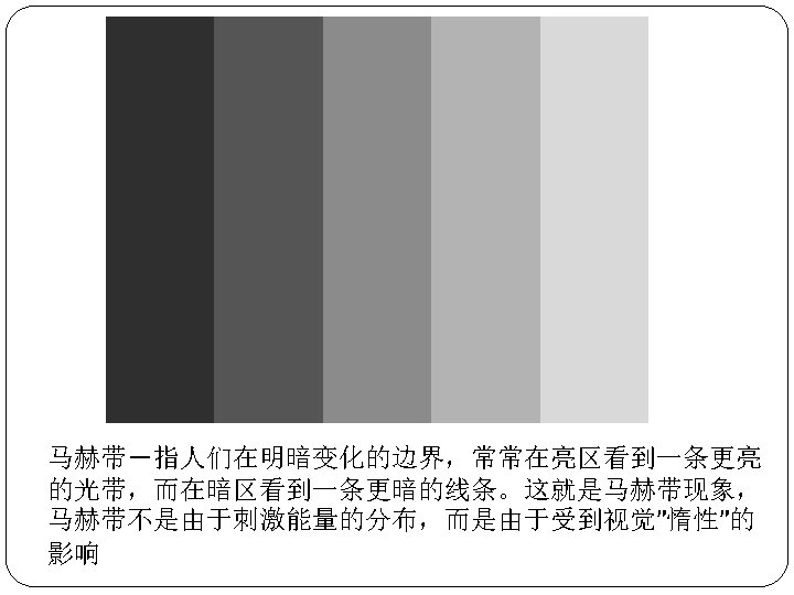
What is Saliency map? �The Saliency Map is a topographically arranged map that represents visual saliency of a corresponding visual scene.

How to detect Saliency map? �Buttom-up approach �L. Itti’s approach �Spectral Residual approach �Frequency-tuned approach �Global contrast based approach �Top-down approach �Context-aware

How to detect Saliency map? �Button-up approach �L. Itti’s approach �Spectral Residual approach �Frequency-tuned approach �Global contrast based approach �Top-down approach �Context-aware

L. Itti’s approach (TPAMI, 1998) Gaussian Pyramids R, G, B, Y Gabor pyramids for q = {0º, 45º, 90º, 135º}

Gaussian Pyramid

Gabor Filter �Gabor filter, is a linear filter used for edge detection, texture representation and discrimination. �In the spatial domain, a 2 D Gabor filter is a Gaussian kernel function modulated by a sinusoidal plane wave. �J. G. Daugman discovered that simple cells in the visual cortex of mammalian brains can be modeled by Gabor functions. Thus, image analysis by the Gabor functions is similar to perception in the human visual system.

Gabor Filter

L. Itti’s approach (TPAMI, 1998) Gaussian Pyramids R, G, B, Y Gabor pyramids for q = {0º, 45º, 90º, 135º}

L. Itti’s approach (TPAMI, 1998) Gaussian Pyramids R, G, B, Y Gabor pyramids for q = {0º, 45º, 90º, 135º}

Laplacian of Gaussian (LOG) �

Relations between DOG and LOG �

L. Itti’s approach (TPAMI, 1998) � Center-surround Difference � Achieve center-surround difference through across-scale difference � Operated denoted by Q: Interpolation to finer scale and point-to- point subtraction � One pyramid for each channel: I(s), R(s), G(s), B(s), Y(s) where s Î [0. . 8] is the scale

L. Itti’s approach (TPAMI, 1998) �Center-surround Difference �Intensity Feature Maps �I(c, s) = | I(c) Q I(s)| �c Î {2, 3, 4} �s = c + d where d Î {3, 4} �So I(2, 5) = | I(2) Q I(5)| I(2, 6) = | I(2) Q I(6)| I(3, 6) = | I(3) Q I(6)| … � 6 Feature Maps

L. Itti’s approach (TPAMI, 1998) Center-surround Difference • l • Color Feature Maps Red-Green and Yellow-Blue l Orientation Feature Maps � Same c and s as with intensity +B-Y +R-G +G-R +R-G +B-Y +Y-B +B-Y RG(c, s) = | (R(c) - G(c)) Q (G(s) - R(s)) | BY(c, s) = | (B(c) - Y(c)) Q (Y(s) - B(s)) |

L. Itti’s approach (TPAMI, 1998) � Normalization Operator � Promotes maps with few strong peaks � Surpresses maps with many comparable peaks

L. Itti’s approach (TPAMI, 1998) Inhibition of return

How to detect Saliency map? �Button-up approach �L. Itti’s approach �Spectral Residual approach �Frequency-tuned approach �Global contrast based approach �Top-down approach �Context-aware

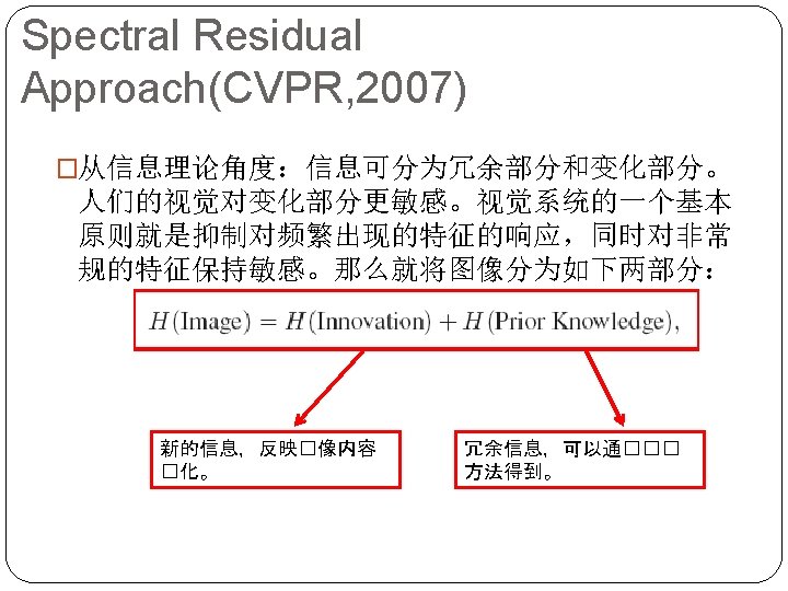
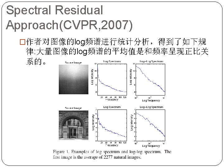
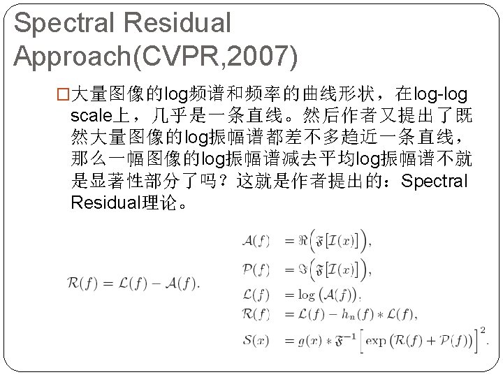
Spectral Residual Approach(CVPR, 2007) �First scaling image to 64 x 64. �hn(f) is a local average filter (n=3 in this paper). �Then the saliency map is smoothed with a gaussian filter g(x) ( σ = 8).

Spectral Residual Approach(CVPR, 2007)

Spectral Residual Approach(CVPR, 2007) clear Clc %% Read image from file in. Img = im 2 double(rgb 2 gray(imread('256. png'))); %%in. Img = imresize(in. Img, 64/size(in. Img, 2)); %% Spectral Residual my. FFT = fft 2(in. Img); my. Log. Amplitude = log(abs(my. FFT)); my. Phase = angle(my. FFT); my. Spectral. Residual = my. Log. Amplitude - imfilter(my. Log. Amplitude, fspecial('average', 3), 'replicate'); saliency. Map = abs(ifft 2(exp(my. Spectral. Residual + i*my. Phase))). ^2; %% After Effect saliency. Map = mat 2 gray(imfilter(saliency. Map, fspecial('gaussian', [10, 10], 2. 5))); imshow(saliency. Map);

How to detect Saliency map? �Button-up approach �L. Itti’s approach �Spectral Residual approach �Frequency-tuned approach �Global contrast based approach �Top-down approach �Context-aware

Frequency-tuned (CVPR, 2009)

Frequency-tuned (CVPR, 2009) �Set the following requirements for a saliency detector: � Emphasize the largest salient objects. � Uniformly highlight whole salient regions. � Establish well-defined boundaries of salient objects. � Disregard high frequencies arising from texture, noise and blocking artifacts. � Efficiently output full resolution saliency maps.

Frequency-tuned (CVPR, 2009) �Choose the Do. G filter for band pass filtering. �Parameter selection �To implement a large ratio in standard deviations, σ1 is driven to infinity.

Frequency-tuned (CVPR, 2009) Image Average Gaussian blur

Frequency-tuned (CVPR, 2009)

Frequency-tuned (CVPR, 2009) % Read image and blur it with a 3 x 3 or 5 x 5 Gaussian filter img = imread('input_image. jpg'); %Provide input image path gfrgb = imfilter(img, fspecial(‘gaussian’, 3, 3), ‘symmetric’, ‘conv’); % Perform s. RGB to CIE Lab color space conversion (using D 65) cform = makecform('srgb 2 lab', 'whitepoint', whitepoint('d 65')); lab = applycform(gfrgb, cform); % Compute Lab average values (note that in the paper this % average is found from the unblurred original image, but the results are quite similar) l = double(lab(: , 1)); lm = mean(l)); a = double(lab(: , 2)); am = mean(a)); b = double(lab(: , 3)); bm = mean(b)); % Finally compute the saliency map and display it. sm = (l-lm). ^2 + (a-am). ^2 + (b-bm). ^2;

How to detect Saliency map? �Button-up approach �L. Itti’s approach �Spectral Residual approach �Frequency-tuned approach �Global contrast based approach �Top-down approach �Context-aware

Global contrast-based (CVPR, 2011)

Global contrast-based (CVPR, 2011) � RC based saliency Cut achieves P = 90%, R = 90%, compared to previous best results P = 75%, R = 83% on this dataset. � P = Precision; R = Recall.

How to detect Saliency map? �Button-up approach �L. Itti’s approach �Spectral Residual approach �Frequency-tuned approach �Global contrast based approach �Top-down approach �Context-aware

Context-Aware (CVPR, 2010) �Goal: 52 Convey the image content

Context-Aware (CVPR, 2010) �Principles of context-aware saliency: � 1. Local low-level considerations, including factors such as contrast and color. � 2. Global considerations, which suppress frequently occurring features, while maintaining features that deviate from the norm. � 3. Visual organization rules, which state that visual forms may possess one or several centers of gravity about which the form is organized. � 4. High-level factors, such as human faces. 53

Context-Aware (CVPR, 2010) �Distance between a pair of patches: High salient

Context-Aware (CVPR, 2010) �Distance between a pair of patches: K most similar patches at scale r High for K most similar Saliency

Context-Aware (CVPR, 2010) �Salient at: �Multiple scales foreground �Few scales background Scale 1 Scale 4

Context-Aware (CVPR, 2010) �Foci = �Include distance map X

Context-Aware (CVPR, 2010) �High-level factors: �The saliency map should be further enhanced using some high-level factors, such as recognized objects or face detection. �In this paper, the face detection algorithm is incorporated , which generates 1 for face pixels and 0 otherwise. �The saliency map is modified by taking the maximum value of the saliency map and the face map.

Is bottom-up attention useful for object recognition? (CVPR, 2004) � This paper investigate empirically to what extent pure bottom-up attention can extract useful information about the location, size and shape of objects from images and demonstrate how this information can be utilized to enable unsupervised learning of objects from unlabeled images. � The experiments demonstrate that the proposed approach to

Saliency-based Object Recognition in 3 D Data (IROS, 2004)