Lecture 12 more Chapter 5 Section 3 Relationships

Lecture 12: more Chapter 5, Section 3 Relationships between Two Quantitative Variables; Regression o. Equation of Regression Line; Residuals o. Effect of Explanatory/Response Roles o. Unusual Observations o. Sample vs. Population o. Time Series; Additional Variables © 2011 Brooks/Cole, Cengage Learning Elementary Statistics: Looking at the Big Picture 1

Looking Back: Review o 4 Stages of Statistics n n Data Production (discussed in Lectures 1 -4) Displaying and Summarizing o o Single variables: 1 cat, 1 quan (discussed Lectures 5 -8) Relationships between 2 variables: n n n Categorical and quantitative (discussed in Lecture 9) Two categorical (discussed in Lecture 10) Two quantitative Probability Statistical Inference © 2011 Brooks/Cole, Cengage Learning Elementary Statistics: Looking at the Big Picture L 12. 2

Review o Relationship between 2 quantitative variables n n Display with scatterplot Summarize: Form: linear or curved o Direction: positive or negative o Strength: strong, moderate, weak If form is linear, correlation r tells direction and strength. Also, equation of least squares regression line lets us predict a response for any explanatory value x. o © 2011 Brooks/Cole, Cengage Learning Elementary Statistics: Looking at the Big Picture L 12. 3

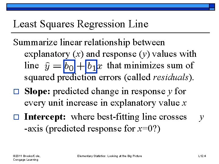
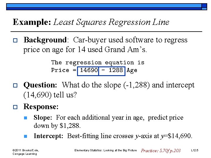
Least Squares Regression Line Summarize linear relationship between explanatory (x) and response (y) values with line that minimizes sum of squared prediction errors (called residuals). o Slope: predicted change in response y for every unit increase in explanatory value x o Intercept: where best-fitting line crosses y -axis (predicted response for x=0? ) © 2011 Brooks/Cole, Cengage Learning Elementary Statistics: Looking at the Big Picture L 12. 4

Example: Least Squares Regression Line o Background: Car-buyer used software to regress price on age for 14 used Grand Am’s. o Question: What do the slope (-1, 288) and intercept (14, 690) tell us? Response: o n n Slope: For each additional year in age, predict price down by $1, 288. Intercept: Best-fitting line crosses y-axis at y=$14, 690. © 2011 Brooks/Cole, Cengage Learning Elementary Statistics: Looking at the Big Picture Practice: 5. 70 f p. 203 L 12. 5

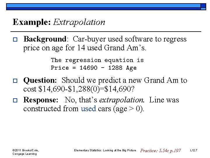
Example: Extrapolation o Background: Car-buyer used software to regress price on age for 14 used Grand Am’s. o Question: Should we predict a new Grand Am to cost $14, 690 -$1, 288(0)=$14, 690? Response: No, that’s extrapolation. Line was constructed from used cars (age > 0). o © 2011 Brooks/Cole, Cengage Learning Elementary Statistics: Looking at the Big Picture Practice: 5. 54 c p. 197 L 12. 7

Definition o Extrapolation: using the regression line to predict responses for explanatory values outside the range of those used to construct the line. © 2011 Brooks/Cole, Cengage Learning Elementary Statistics: Looking at the Big Picture L 12. 9

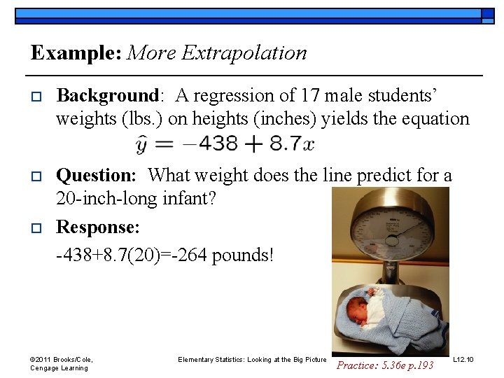
Example: More Extrapolation o Background: A regression of 17 male students’ weights (lbs. ) on heights (inches) yields the equation o Question: What weight does the line predict for a 20 -inch-long infant? Response: -438+8. 7(20)=-264 pounds! o © 2011 Brooks/Cole, Cengage Learning Elementary Statistics: Looking at the Big Picture Practice: 5. 36 e p. 193 L 12. 10

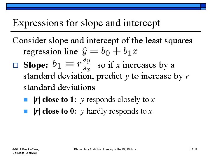
Expressions for slope and intercept Consider slope and intercept of the least squares regression line o Slope: so if x increases by a standard deviation, predict y to increase by r standard deviations n n |r| close to 1: y responds closely to x |r| close to 0: y hardly responds to x © 2011 Brooks/Cole, Cengage Learning Elementary Statistics: Looking at the Big Picture L 12. 12

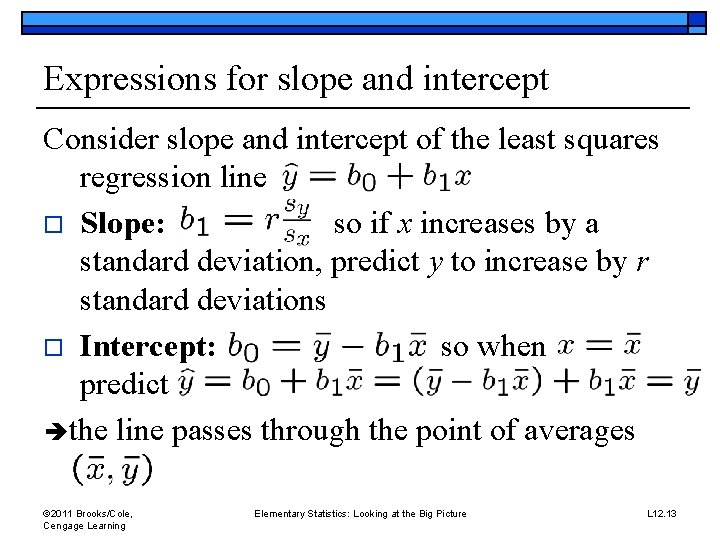
Expressions for slope and intercept Consider slope and intercept of the least squares regression line o Slope: so if x increases by a standard deviation, predict y to increase by r standard deviations o Intercept: so when predict the line passes through the point of averages © 2011 Brooks/Cole, Cengage Learning Elementary Statistics: Looking at the Big Picture L 12. 13

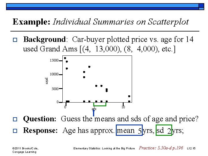
Example: Individual Summaries on Scatterplot o Background: Car-buyer plotted price vs. age for 14 used Grand Ams [(4, 13, 000), (8, 4, 000), etc. ] 15000 10000 price 5000 0 0 o o 5 age 10 Question: Guess the means and sds of age and price? Response: Age has approx. mean 5 yrs, sd 2 yrs; © 2011 Brooks/Cole, Cengage Learning Elementary Statistics: Looking at the Big Picture Practice: 5. 50 a-d p. 196 L 12. 15

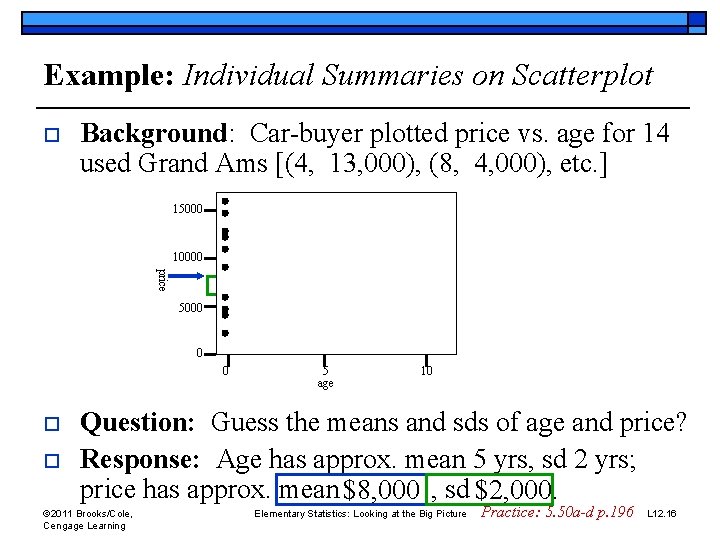
Example: Individual Summaries on Scatterplot o Background: Car-buyer plotted price vs. age for 14 used Grand Ams [(4, 13, 000), (8, 4, 000), etc. ] 15000 10000 price 5000 0 0 o o 5 age 10 Question: Guess the means and sds of age and price? Response: Age has approx. mean 5 yrs, sd 2 yrs; price has approx. mean $8, 000 , sd $2, 000. © 2011 Brooks/Cole, Cengage Learning Elementary Statistics: Looking at the Big Picture Practice: 5. 50 a-d p. 196 L 12. 16

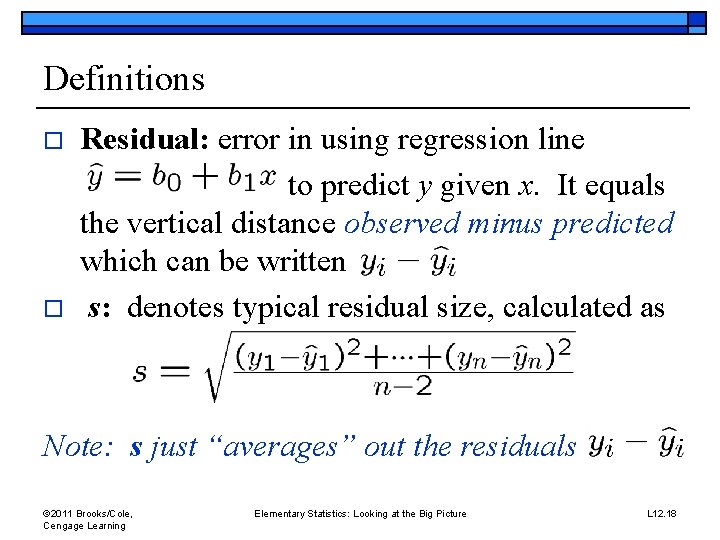
Definitions o o Residual: error in using regression line to predict y given x. It equals the vertical distance observed minus predicted which can be written s: denotes typical residual size, calculated as Note: s just “averages” out the residuals © 2011 Brooks/Cole, Cengage Learning Elementary Statistics: Looking at the Big Picture L 12. 18

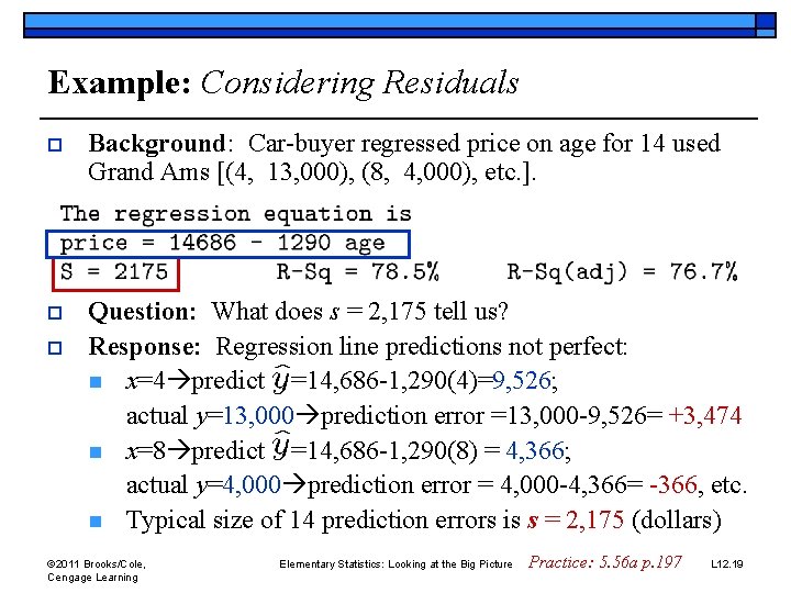
Example: Considering Residuals o Background: Car-buyer regressed price on age for 14 used Grand Ams [(4, 13, 000), (8, 4, 000), etc. ]. o Question: What does s = 2, 175 tell us? Response: Regression line predictions not perfect: n x=4 predict =14, 686 -1, 290(4)=9, 526; actual y=13, 000 prediction error =13, 000 -9, 526= +3, 474 n x=8 predict =14, 686 -1, 290(8) = 4, 366; actual y=4, 000 prediction error = 4, 000 -4, 366= -366, etc. n Typical size of 14 prediction errors is s = 2, 175 (dollars) o © 2011 Brooks/Cole, Cengage Learning Elementary Statistics: Looking at the Big Picture Practice: 5. 56 a p. 197 L 12. 19

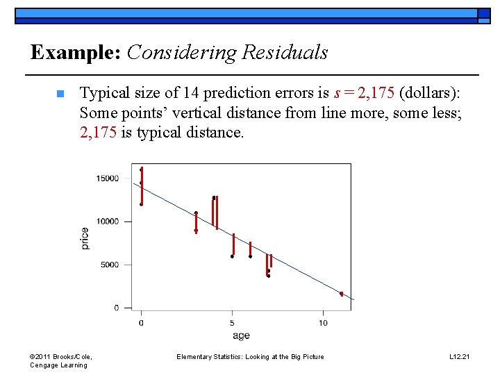
Example: Considering Residuals n Typical size of 14 prediction errors is s = 2, 175 (dollars): Some points’ vertical distance from line more, some less; 2, 175 is typical distance. © 2011 Brooks/Cole, Cengage Learning Elementary Statistics: Looking at the Big Picture L 12. 21

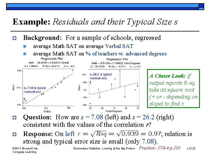
Example: Residuals and their Typical Size s o Background: For a sample of schools, regressed n n average Math SAT on average Verbal SAT average Math SAT on % of teachers w. advanced degrees A Closer Look: If output reports R-sq, take its square root (+ or - depending on slope) to find r. o o Question: How are s = 7. 08 (left) and s = 26. 2 (right) consistent with the values of the correlation r? Response: On left ; relation is strong and typical error size is small (only 7. 08). © 2011 Brooks/Cole, Cengage Learning Elementary Statistics: Looking at the Big Picture Practice: 570 i-k p. 203 L 12. 22

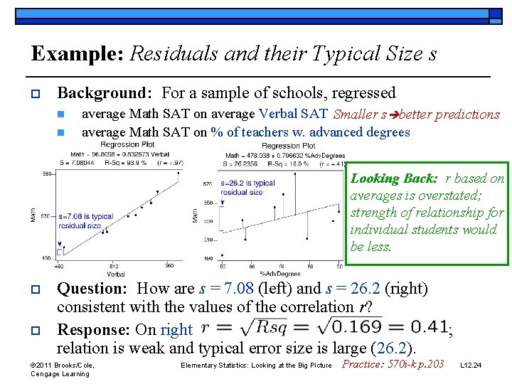
Example: Residuals and their Typical Size s o Background: For a sample of schools, regressed n n average Math SAT on average Verbal SAT Smaller s better predictions average Math SAT on % of teachers w. advanced degrees Looking Back: r based on averages is overstated; strength of relationship for individual students would be less. o o Question: How are s = 7. 08 (left) and s = 26. 2 (right) consistent with the values of the correlation r? Response: On right relation is weak and typical error size is large (26. 2). © 2011 Brooks/Cole, Cengage Learning Elementary Statistics: Looking at the Big Picture Practice: 570 i-k p. 203 ; L 12. 24

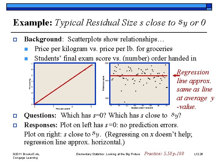
Example: Typical Residual Size s close to o or 0 Background: Scatterplots show relationships… n Price per kilogram vs. price per lb. for groceries n Students’ final exam score vs. (number) order handed in Regression line approx. same as line at average y -value. Questions: Which has s=0? Which has s close to ? Responses: Plot on left has s=0: no prediction errors. Plot on right: s close to. (Regressing on x doesn’t help; regression line approx. horizontal. ) © 2011 Brooks/Cole, Cengage Learning Elementary Statistics: Looking at the Big Picture Practice: 5. 58 p. 198 L 12. 26

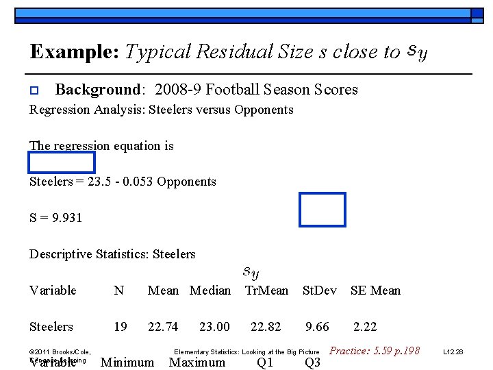
Example: Typical Residual Size s close to o Background: 2008 -9 Football Season Scores Regression Analysis: Steelers versus Opponents The regression equation is Steelers = 23. 5 - 0. 053 Opponents S = 9. 931 Descriptive Statistics: Steelers Variable N Mean Median Steelers 19 22. 74 © 2011 Brooks/Cole, Cengage Learning Variable Minimum 23. 00 Tr. Mean St. Dev SE Mean 22. 82 9. 66 2. 22 Elementary Statistics: Looking at the Big Picture Maximum Q 1 Q 3 Practice: 5. 59 p. 198 L 12. 28

Explanatory/Response Roles in Regression Our choice of roles, explanatory or response, does not affect the value of the correlation r, but it does affect the regression line. © 2011 Brooks/Cole, Cengage Learning Elementary Statistics: Looking at the Big Picture L 12. 30

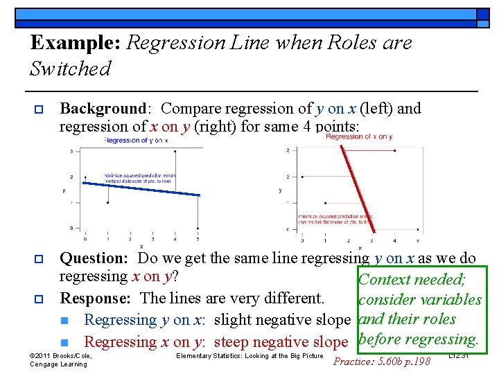
Example: Regression Line when Roles are Switched o Background: Compare regression of y on x (left) and regression of x on y (right) for same 4 points: o Question: Do we get the same line regressing y on x as we do regressing x on y? Context needed; Response: The lines are very different. consider variables n Regressing y on x: slight negative slope and their roles n Regressing x on y: steep negative slope before regressing. o © 2011 Brooks/Cole, Cengage Learning Elementary Statistics: Looking at the Big Picture Practice: 5. 60 b p. 198 L 12. 31

Definitions o o Outlier: (in regression) point with unusually large residual Influential observation: point with high degree of influence on regression line. © 2011 Brooks/Cole, Cengage Learning Elementary Statistics: Looking at the Big Picture L 12. 33

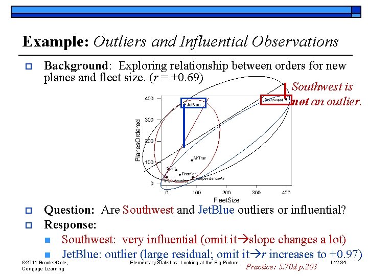
Example: Outliers and Influential Observations o Background: Exploring relationship between orders for new planes and fleet size. (r = +0. 69) Southwest is not an outlier. o Question: Are Southwest and Jet. Blue outliers or influential? Response: n Southwest: very influential (omit it slope changes a lot) n Jet. Blue: outlier (large residual; omit it r increases to +0. 97) o © 2011 Brooks/Cole, Cengage Learning Elementary Statistics: Looking at the Big Picture Practice: 5. 70 d p. 203 L 12. 34

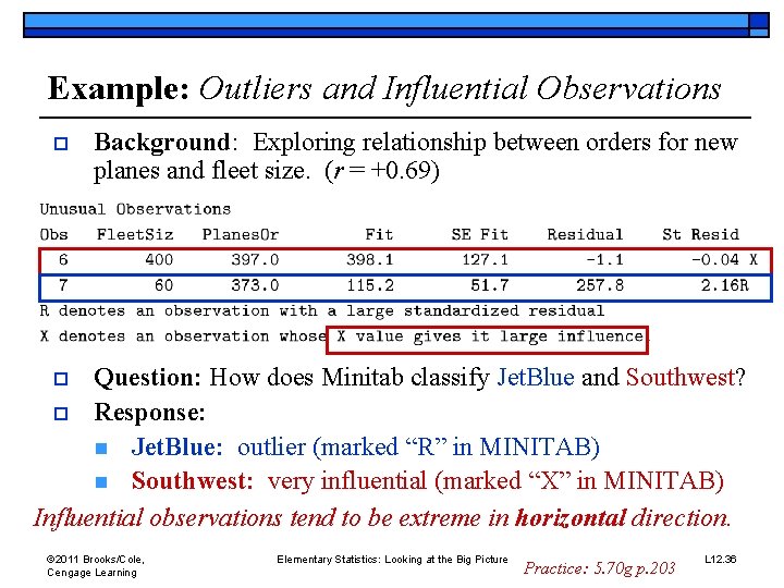
Example: Outliers and Influential Observations o Background: Exploring relationship between orders for new planes and fleet size. (r = +0. 69) Question: How does Minitab classify Jet. Blue and Southwest? o Response: n Jet. Blue: outlier (marked “R” in MINITAB) n Southwest: very influential (marked “X” in MINITAB) Influential observations tend to be extreme in horizontal direction. o © 2011 Brooks/Cole, Cengage Learning Elementary Statistics: Looking at the Big Picture Practice: 5. 70 g p. 203 L 12. 36

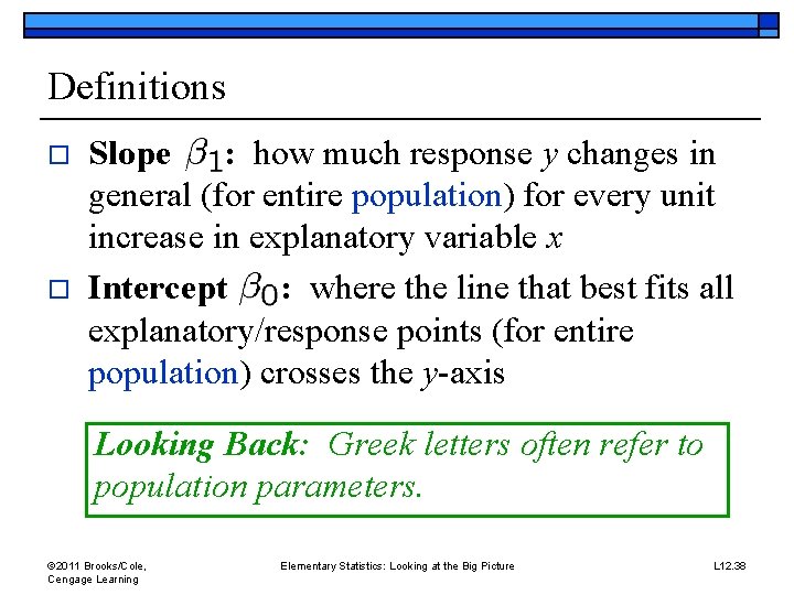
Definitions o o Slope : how much response y changes in general (for entire population) for every unit increase in explanatory variable x Intercept : where the line that best fits all explanatory/response points (for entire population) crosses the y-axis Looking Back: Greek letters often refer to population parameters. © 2011 Brooks/Cole, Cengage Learning Elementary Statistics: Looking at the Big Picture L 12. 38

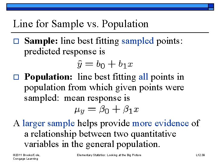
Line for Sample vs. Population o Sample: line best fitting sampled points: predicted response is o Population: line best fitting all points in population from which given points were sampled: mean response is A larger sample helps provide more evidence of a relationship between two quantitative variables in the general population. © 2011 Brooks/Cole, Cengage Learning Elementary Statistics: Looking at the Big Picture L 12. 39

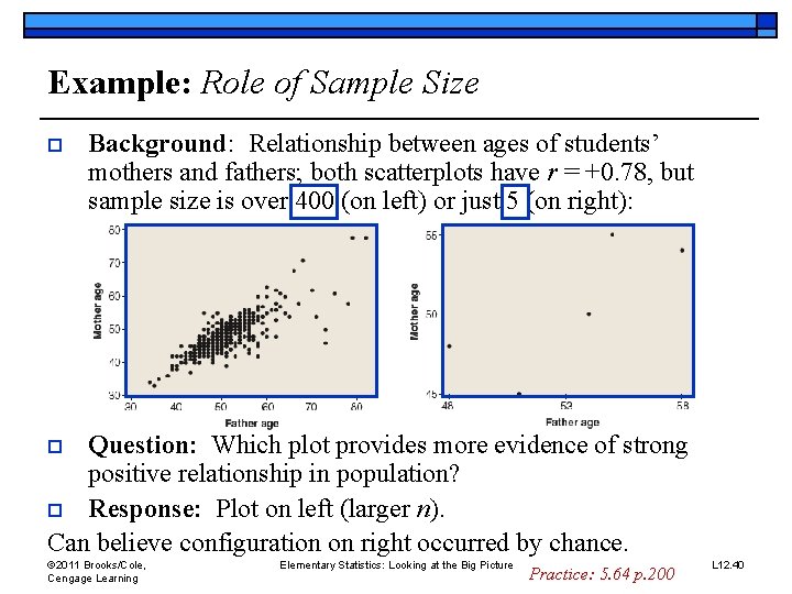
Example: Role of Sample Size o Background: Relationship between ages of students’ mothers and fathers; both scatterplots have r = +0. 78, but sample size is over 400 (on left) or just 5 (on right): Question: Which plot provides more evidence of strong positive relationship in population? o Response: Plot on left (larger n). Can believe configuration on right occurred by chance. o © 2011 Brooks/Cole, Cengage Learning Elementary Statistics: Looking at the Big Picture Practice: 5. 64 p. 200 L 12. 40

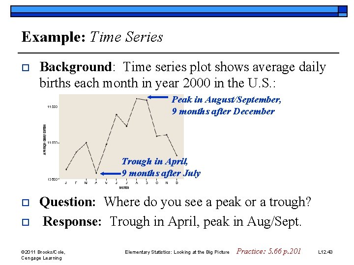
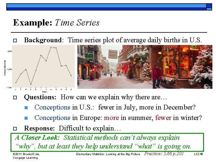
Time Series If explanatory variable is time, plot one response for each time value and “connect the dots” to look for general trend over time, also peaks and troughs. © 2011 Brooks/Cole, Cengage Learning Elementary Statistics: Looking at the Big Picture L 12. 42

Example: Time Series o Background: Time series plot shows average daily births each month in year 2000 in the U. S. : Peak in August/September, 9 months after December Trough in April, 9 months after July o o Question: Where do you see a peak or a trough? Response: Trough in April, peak in Aug/Sept. © 2011 Brooks/Cole, Cengage Learning Elementary Statistics: Looking at the Big Picture Practice: 5. 66 p. 201 L 12. 43

Example: Time Series o Background: Time series plot of average daily births in U. S. Questions: How can we explain why there are… n Conceptions in U. S. : fewer in July, more in December? n Conceptions in Europe: more in summer, fewer in winter? o Response: Difficult to explain… A Closer Look: Statistical methods can’t always explain “why”, but at least they help understand “what” is going on. o © 2011 Brooks/Cole, Cengage Learning Elementary Statistics: Looking at the Big Picture Practice: 5. 66 p. 201 L 12. 45

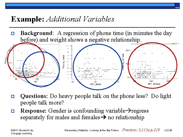
Additional Variables in Regression o o Confounding Variable: Combining two groups that differ with respect to a variable that is related to both explanatory and response variables can affect the nature of their relationship. Multiple Regression: More advanced treatments consider impact of not just one but two or more quantitative explanatory variables on a quantitative response. © 2011 Brooks/Cole, Cengage Learning Elementary Statistics: Looking at the Big Picture L 12. 47

Example: Additional Variables o Background: A regression of phone time (in minutes the day before) and weight shows a negative relationship. o Questions: Do heavy people talk on the phone less? Do light people talk more? Response: Gender is confounding variable regress separately for males and females➔ no relationship o © 2011 Brooks/Cole, Cengage Learning Elementary Statistics: Looking at the Big Picture Practice: 5. 113 a p. 219 L 12. 48

Example: Multiple Regression o o o Background: We used a car’s age to predict its price. Question: What additional quantitative variable would help predict a car’s price? Response: miles driven (among other possibilities) © 2011 Brooks/Cole, Cengage Learning Elementary Statistics: Looking at the Big Picture Practice: 5. 69 b-d p. 201 L 12. 50

Lecture Summary (Regression) o Equation of regression line n n o o o Interpreting slope and intercept Extrapolation Residuals: typical size is s Line affected by explanatory/response roles Outliers and influential observations Line for sample or population; role of sample size Time series Additional variables © 2011 Brooks/Cole, Cengage Learning Elementary Statistics: Looking at the Big Picture L 12. 52