Lecture 12 Economic Growth Economic Growth Explain improvements

Lecture 12 Economic Growth

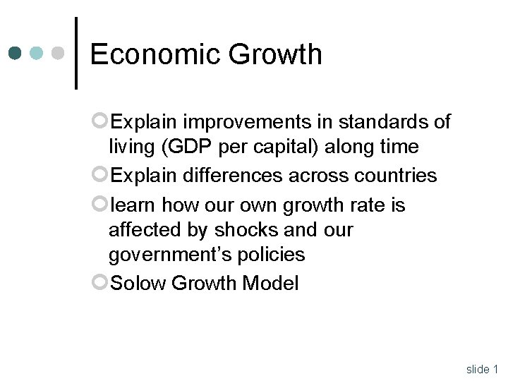
Economic Growth ¢Explain improvements in standards of living (GDP per capital) along time ¢Explain differences across countries ¢learn how our own growth rate is affected by shocks and our government’s policies ¢Solow Growth Model slide 1

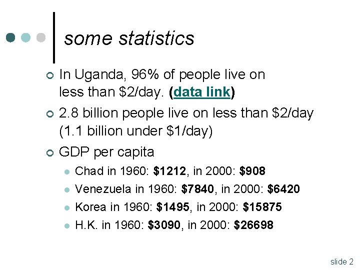
some statistics ¢ In Uganda, 96% of people live on less than $2/day. (data link) ¢ 2. 8 billion people live on less than $2/day (1. 1 billion under $1/day) GDP per capita ¢ l Chad in 1960: $1212, in 2000: $908 l Venezuela in 1960: $7840, in 2000: $6420 Korea in 1960: $1495, in 2000: $15875 H. K. in 1960: $3090, in 2000: $26698 l l slide 2

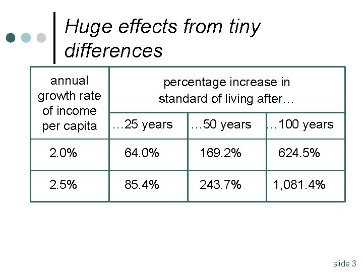
Huge effects from tiny differences annual percentage increase in growth rate standard of living after… of income per capita … 25 years … 50 years … 100 years 2. 0% 64. 0% 169. 2% 624. 5% 2. 5% 85. 4% 243. 7% 1, 081. 4% slide 3

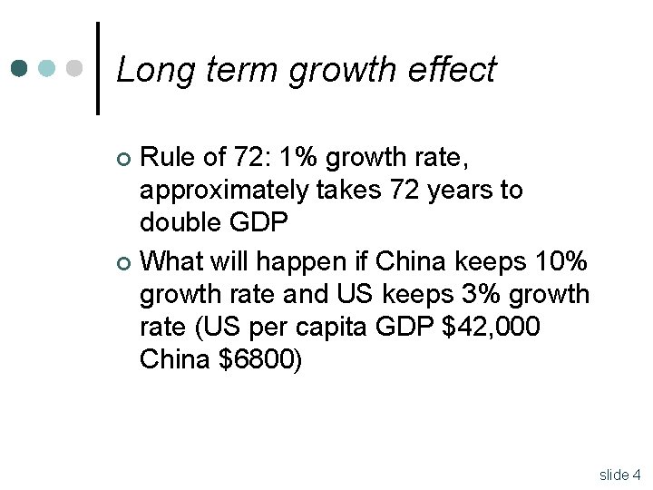
Long term growth effect Rule of 72: 1% growth rate, approximately takes 72 years to double GDP ¢ What will happen if China keeps 10% growth rate and US keeps 3% growth rate (US per capita GDP $42, 000 China $6800) ¢ slide 4

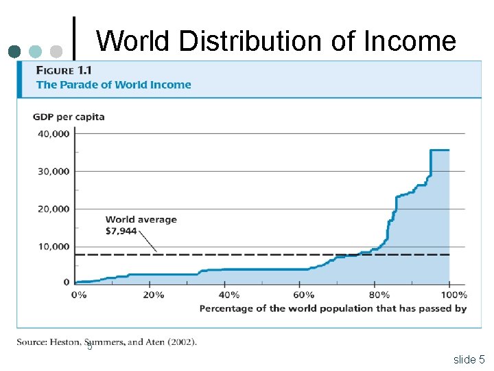
World Distribution of Income 5 slide 5

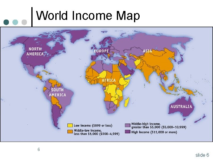
World Income Map 6 slide 6

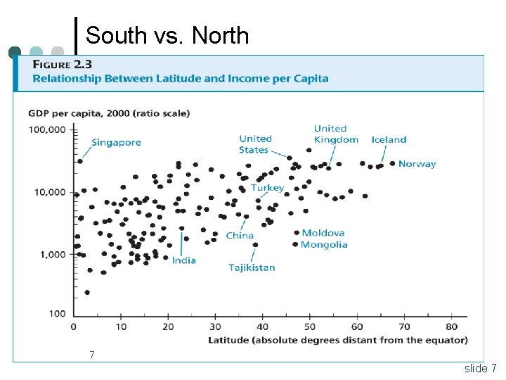
South vs. North 7 slide 7

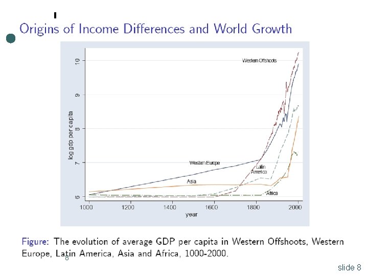
8 slide 8

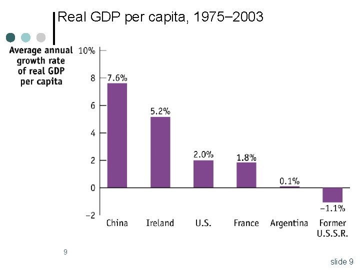
Real GDP per capita, 1975– 2003 9 slide 9

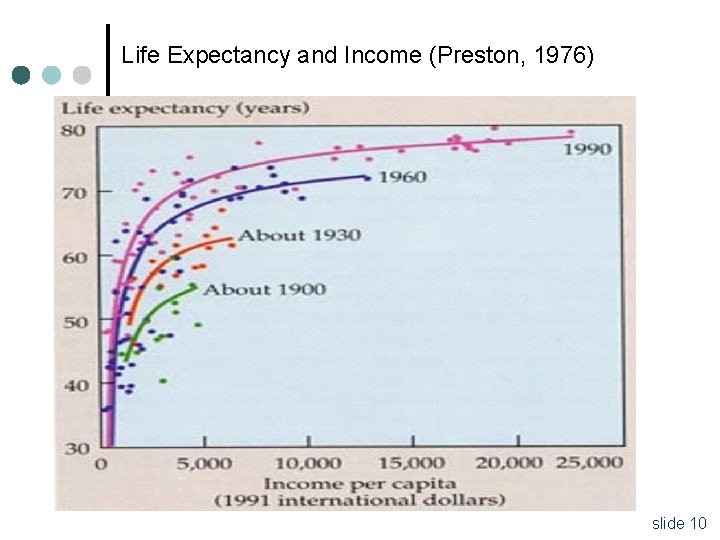
Life Expectancy and Income (Preston, 1976) 10 slide 10

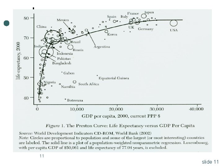
11 slide 11

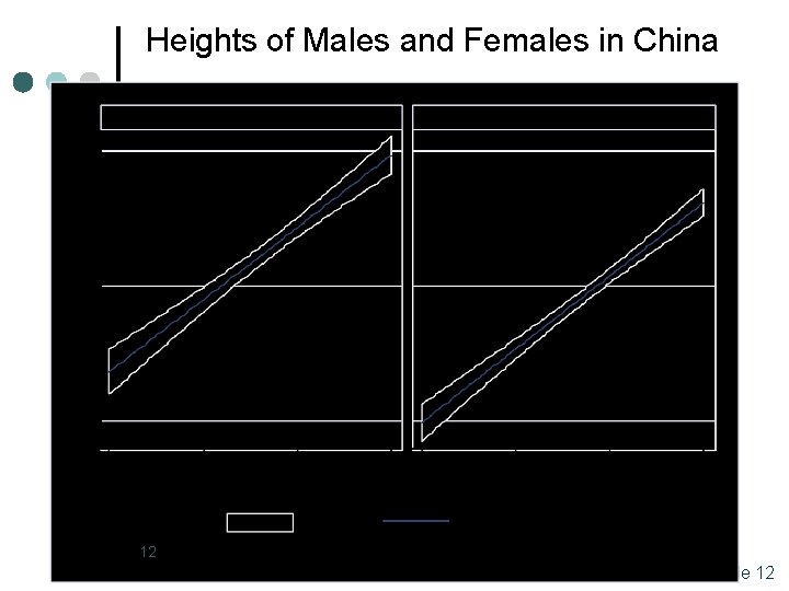
Heights of Males and Females in China 12 slide 12

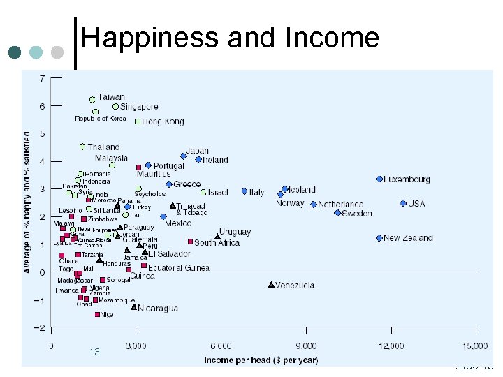
Happiness and Income 13 slide 13

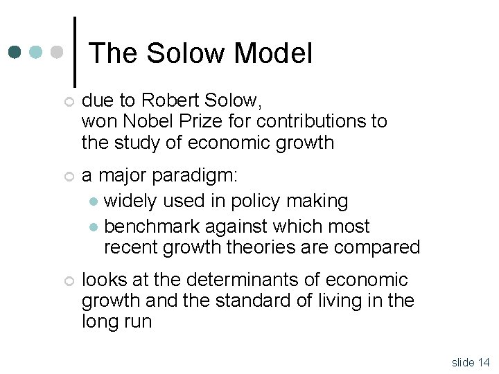
The Solow Model ¢ due to Robert Solow, won Nobel Prize for contributions to the study of economic growth ¢ a major paradigm: l widely used in policy making l benchmark against which most recent growth theories are compared ¢ looks at the determinants of economic growth and the standard of living in the long run slide 14

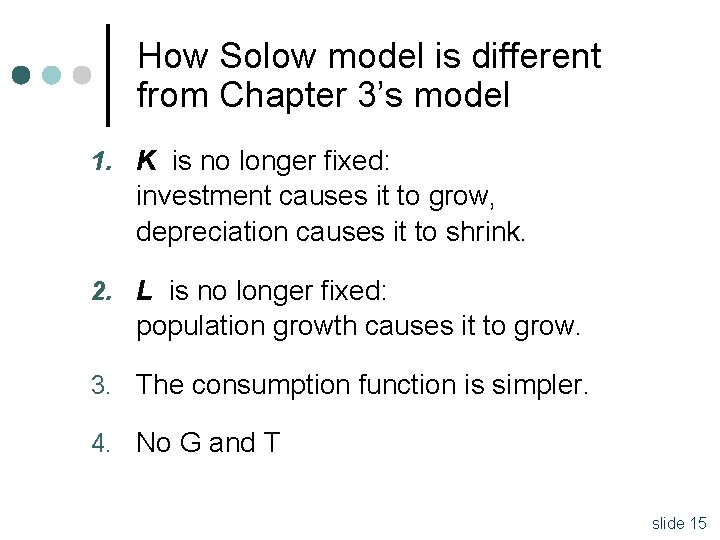
How Solow model is different from Chapter 3’s model 1. K is no longer fixed: investment causes it to grow, depreciation causes it to shrink. 2. L is no longer fixed: population growth causes it to grow. 3. The consumption function is simpler. 4. No G and T slide 15

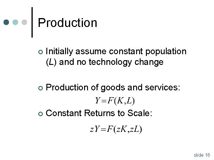
Production ¢ Initially assume constant population (L) and no technology change ¢ Production of goods and services: ¢ Constant Returns to Scale: slide 16

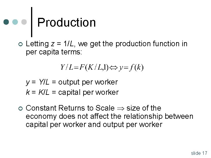
Production ¢ Letting z = 1/L, we get the production function in per capita terms: y = Y/L = output per worker k = K/L = capital per worker ¢ Constant Returns to Scale size of the economy does not affect the relationship between capital per worker and output per worker slide 17

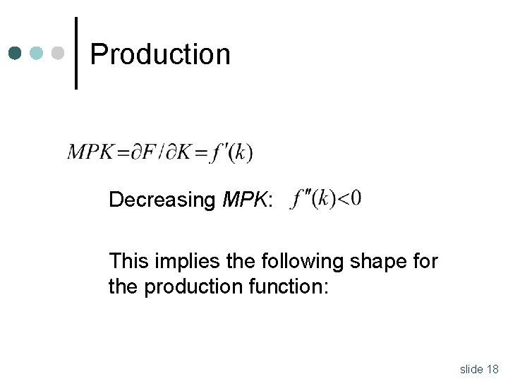
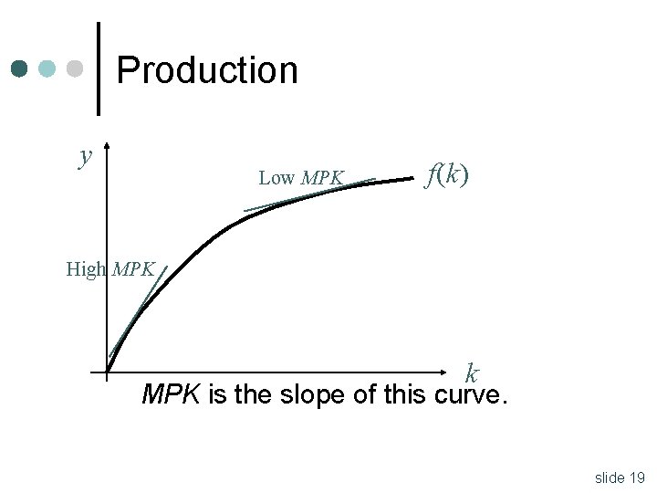
Production Decreasing MPK: This implies the following shape for the production function: slide 18

Production y Low MPK f(k) High MPK k MPK is the slope of this curve. slide 19

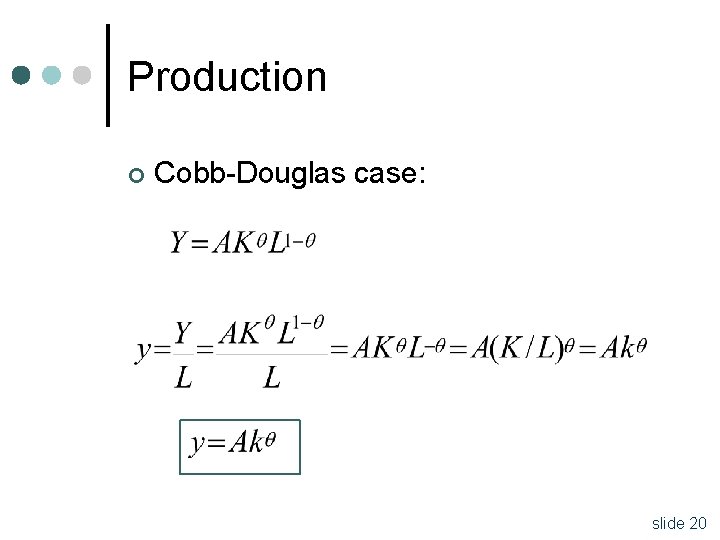
Production ¢ Cobb-Douglas case: slide 20

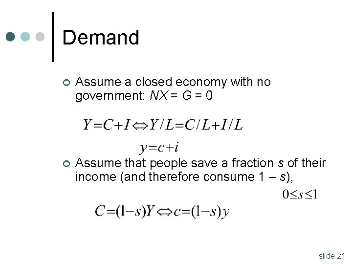
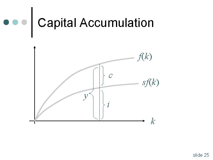
Demand ¢ Assume a closed economy with no government: NX = G = 0 ¢ Assume that people save a fraction s of their income (and therefore consume 1 – s), slide 21

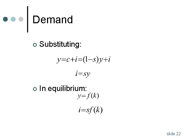
Demand ¢ Substituting: ¢ In equilibrium: slide 22

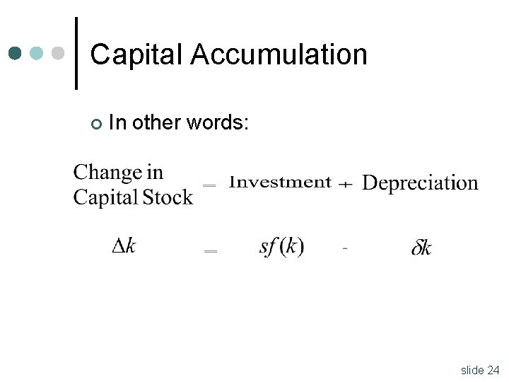
Capital Accumulation ¢ Two elements determine how the capital stock changes over time: Investment: addition of new plants and equipment (makes capital stock rise) l Depreciation: wearing out of existing capital stock (makes capital stock fall) l slide 23

Capital Accumulation ¢ In other words: slide 24

Capital Accumulation f(k) c y sf(k) i k slide 25

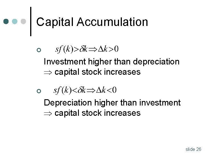
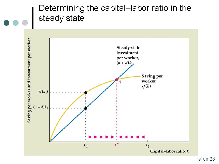
Capital Accumulation ¢ Investment higher than depreciation capital stock increases ¢ Depreciation higher than investment capital stock increases slide 26

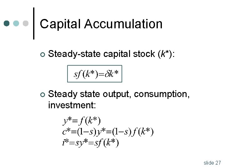
Capital Accumulation ¢ Steady-state capital stock (k*): ¢ Steady state output, consumption, investment: slide 27

Determining the capital–labor ratio in the steady state 28 slide 28

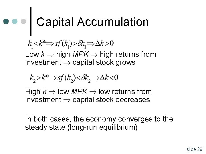
Capital Accumulation Low k high MPK high returns from investment capital stock grows High k low MPK low returns from investment capital stock decreases In both cases, the economy converges to the steady state (long-run equilibrium) slide 29

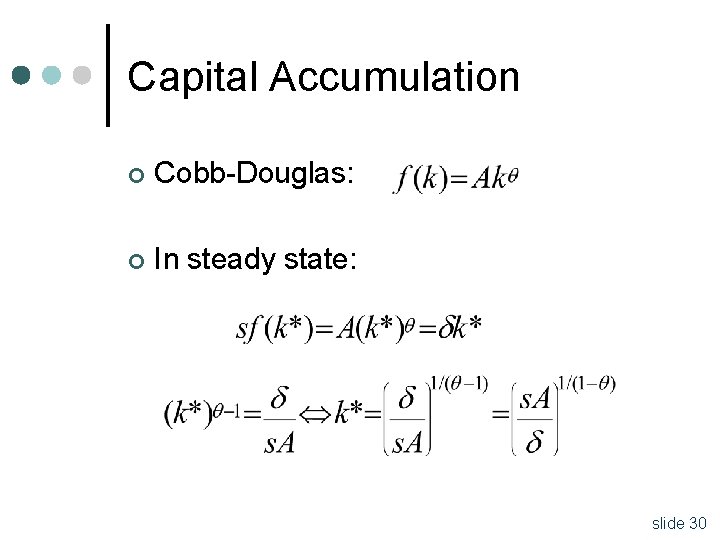
Capital Accumulation ¢ Cobb-Douglas: ¢ In steady state: slide 30

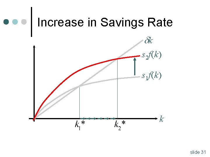
Increase in Savings Rate k s 2 f(k) s 1 f(k) k slide 31

Increase in Savings Rate ¢ Higher s means that more resources will be dedicated to investment higher capital stock in steady state ¢ Therefore, output per capita will be also higher slide 32

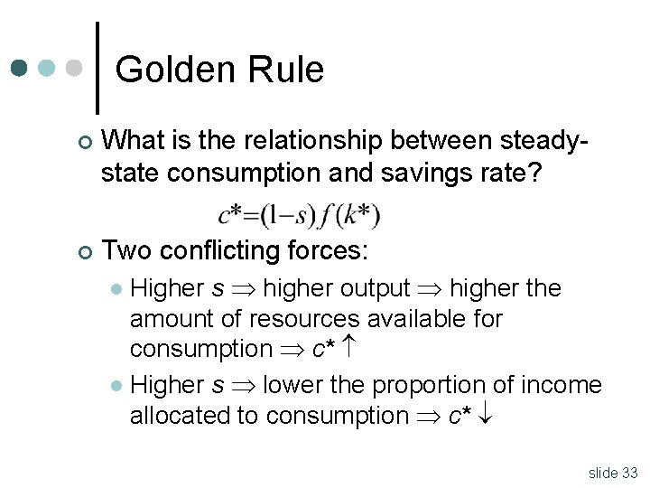
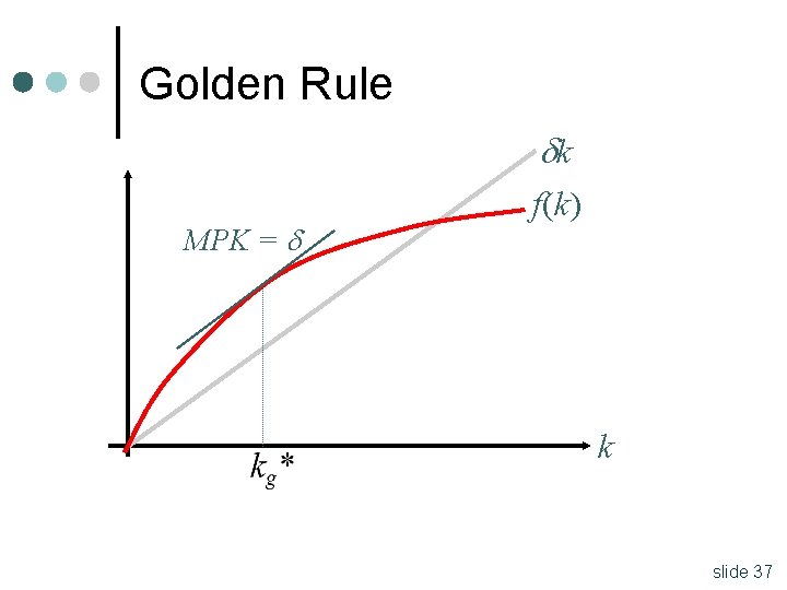
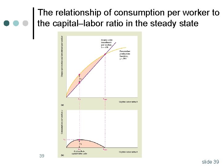
Golden Rule ¢ What is the relationship between steadystate consumption and savings rate? ¢ Two conflicting forces: Higher s higher output higher the amount of resources available for consumption c* l Higher s lower the proportion of income allocated to consumption c* l slide 33

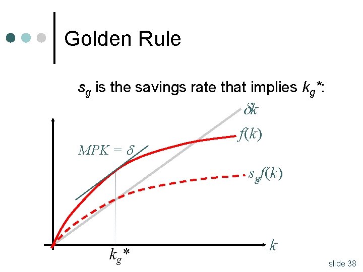
Golden Rule ¢ For low values of s, c* increases with s ¢ For high values of s, c* decreases with s ¢ Golden Rule: capital stock implied by the savings rate such that c* is maximized slide 34

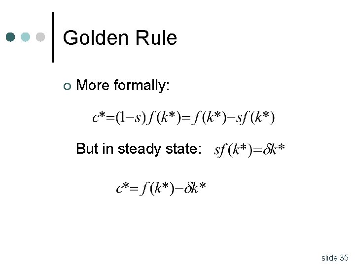
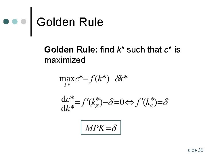
Golden Rule ¢ More formally: But in steady state: slide 35

Golden Rule: find k* such that c* is maximized slide 36

Golden Rule k MPK = f(k) k slide 37

Golden Rule sg is the savings rate that implies kg*: k MPK = f(k) sgf(k) k slide 38

The relationship of consumption per worker to the capital–labor ratio in the steady state 39 slide 39

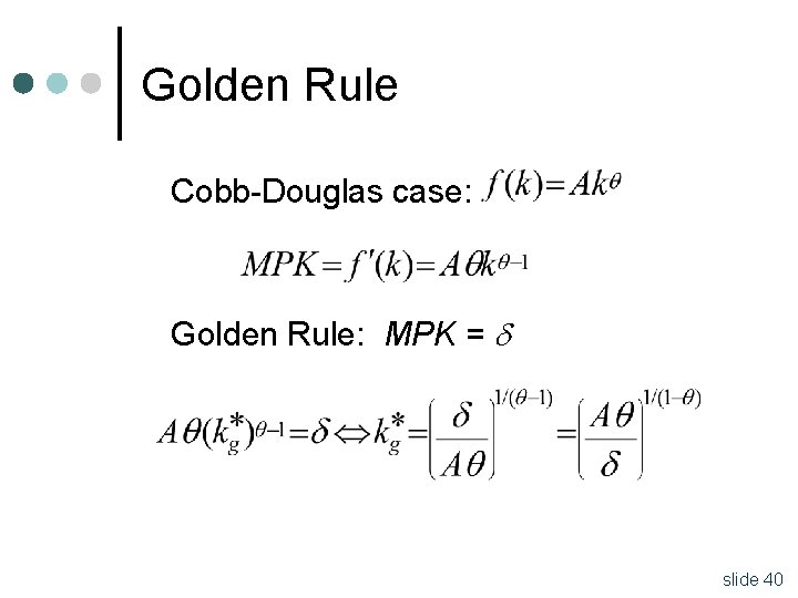
Golden Rule Cobb-Douglas case: Golden Rule: MPK = slide 40

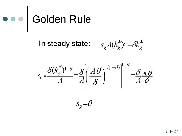
Golden Rule In steady state: slide 41

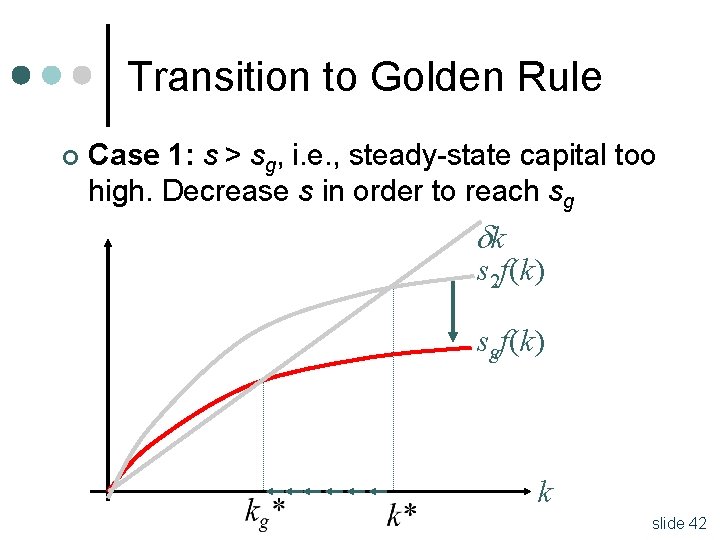
Transition to Golden Rule ¢ Case 1: s > sg, i. e. , steady-state capital too high. Decrease s in order to reach sg k s 2 f(k) sgf(k) k slide 42

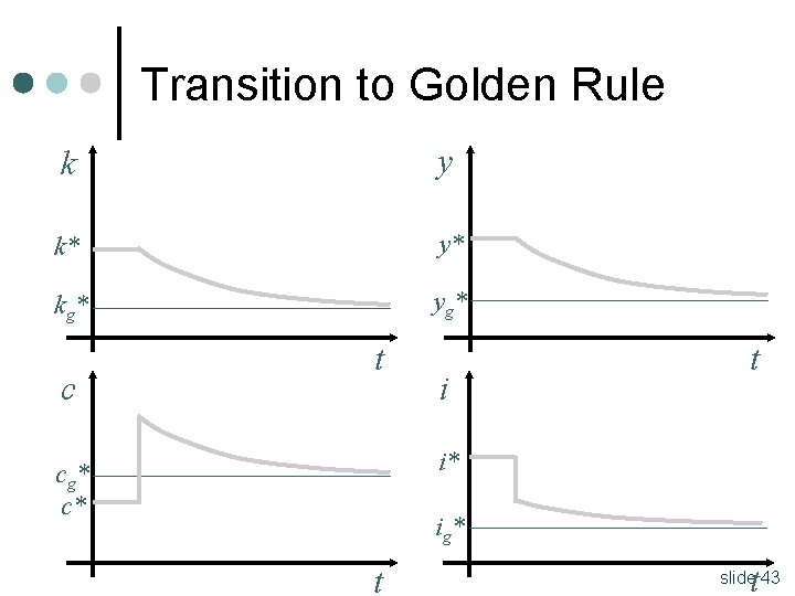
Transition to Golden Rule k y k* y* kg* yg* c t i* cg* c* ig* t t slide 43

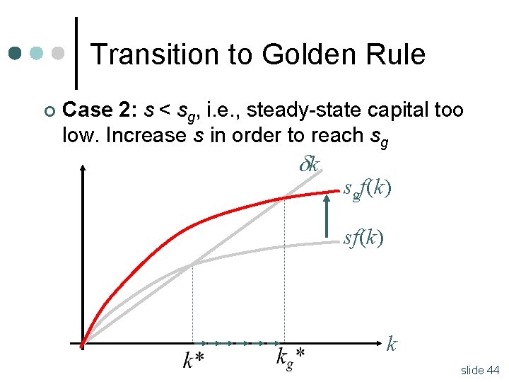
Transition to Golden Rule ¢ Case 2: s < sg, i. e. , steady-state capital too low. Increase s in order to reach sg k sgf(k) sf(k) k slide 44

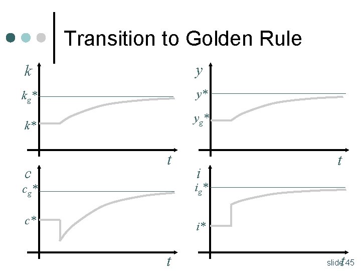
Transition to Golden Rule k y kg* y* k* yg* c t i cg* ig* c* i* t t t slide 45

Transition to Golden Rule ¢ If the economy begins above the golden rule (s too high), consumption increases in all future periods decrease in s leads to welfare improvement ¢ If the economy begins below the golden rule (s too low), consumption falls during transition there is a tradeoff between consuming today or in the future slide 46

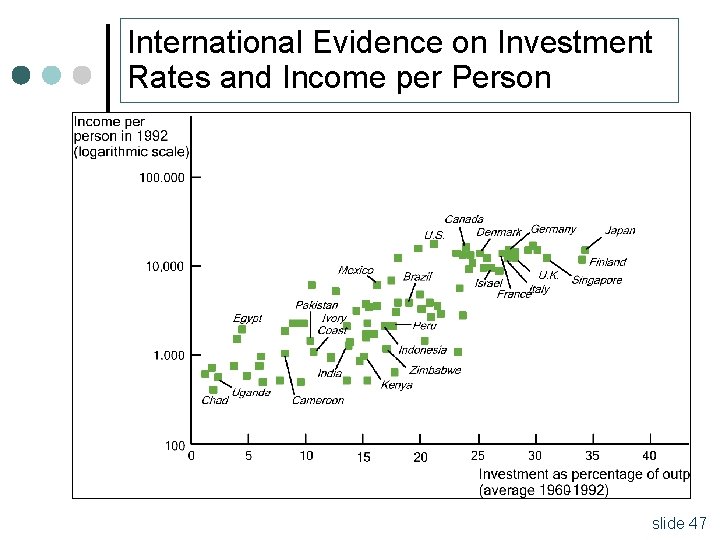
International Evidence on Investment Rates and Income per Person slide 47

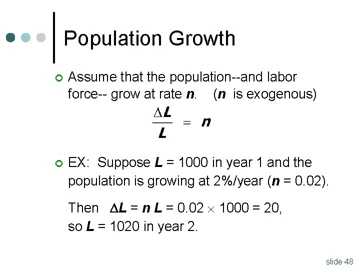
Population Growth ¢ Assume that the population--and labor force-- grow at rate n. (n is exogenous) ¢ EX: Suppose L = 1000 in year 1 and the population is growing at 2%/year (n = 0. 02). Then L = 0. 02 1000 = 20, so L = 1020 in year 2. slide 48

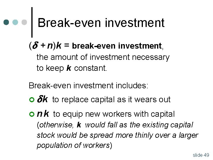
Break-even investment ( + n)k = break-even investment, the amount of investment necessary to keep k constant. Break-even investment includes: ¢ k to replace capital as it wears out ¢ nk to equip new workers with capital (otherwise, k would fall as the existing capital stock would be spread more thinly over a larger population of workers) slide 49

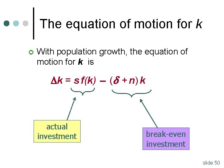
The equation of motion for k ¢ With population growth, the equation of motion for k is k = s f(k) ( + n) k actual investment break-even investment slide 50

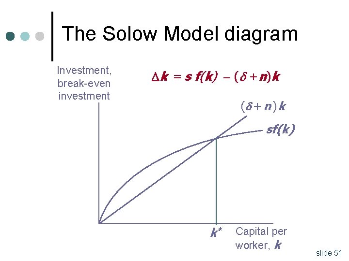
The Solow Model diagram Investment, break-even investment k = s f(k) ( +n)k ( + n ) k sf(k) k* Capital per worker, k slide 51

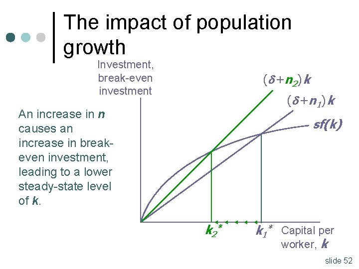
The impact of population growth Investment, break-even investment ( + n 2 ) k ( + n 1 ) k An increase in n causes an increase in breakeven investment, leading to a lower steady-state level of k. sf(k) k 2* k 1* Capital per worker, k slide 52

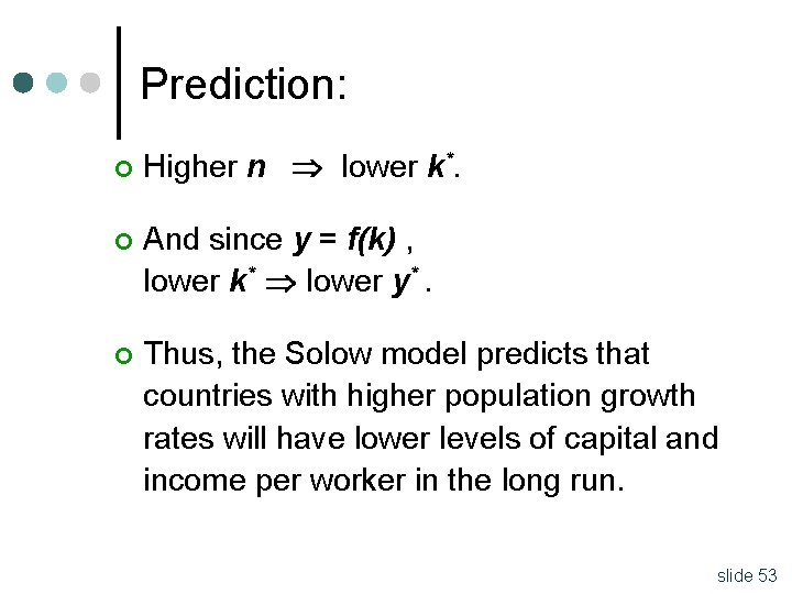
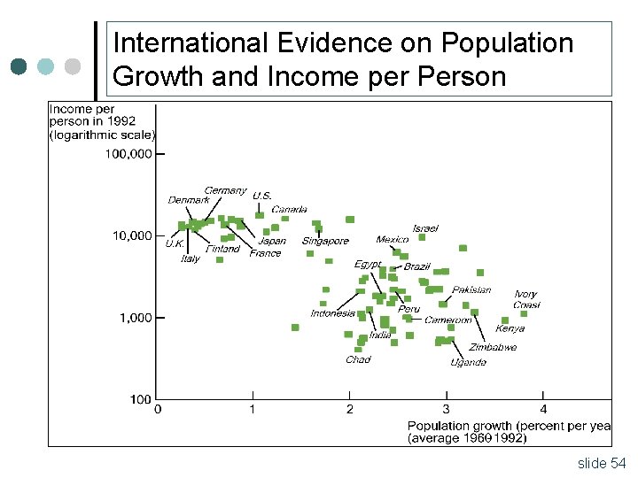
Prediction: ¢ Higher n lower k*. ¢ And since y = f(k) , lower k* lower y*. ¢ Thus, the Solow model predicts that countries with higher population growth rates will have lower levels of capital and income per worker in the long run. slide 53

International Evidence on Population Growth and Income per Person slide 54

55 slide 55

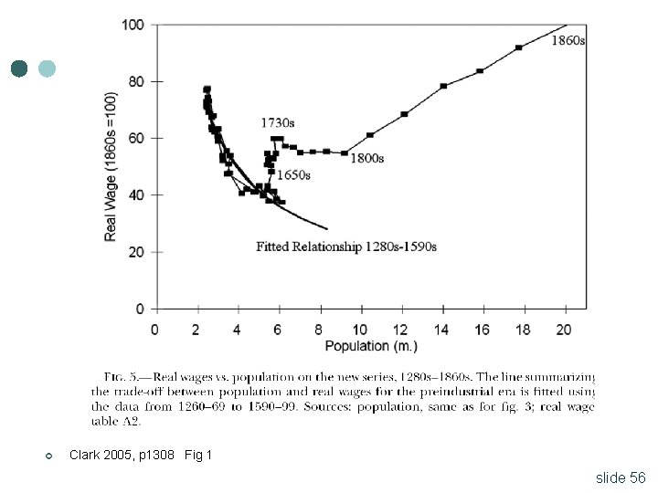
¢ Clark 2005, p 1308 Fig 1 slide 56

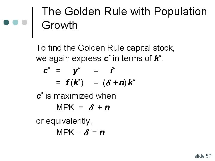
The Golden Rule with Population Growth To find the Golden Rule capital stock, we again express c* in terms of k*: c* = y* i* = f (k* ) ( + n) k* c* is maximized when MPK = + n or equivalently, MPK = n slide 57

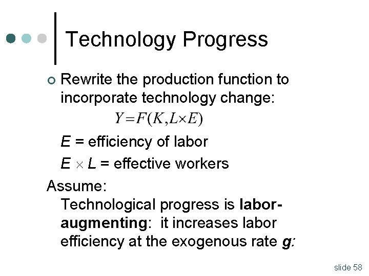
Technology Progress ¢ Rewrite the production function to incorporate technology change: E = efficiency of labor E L = effective workers Assume: Technological progress is laboraugmenting: it increases labor efficiency at the exogenous rate g: slide 58

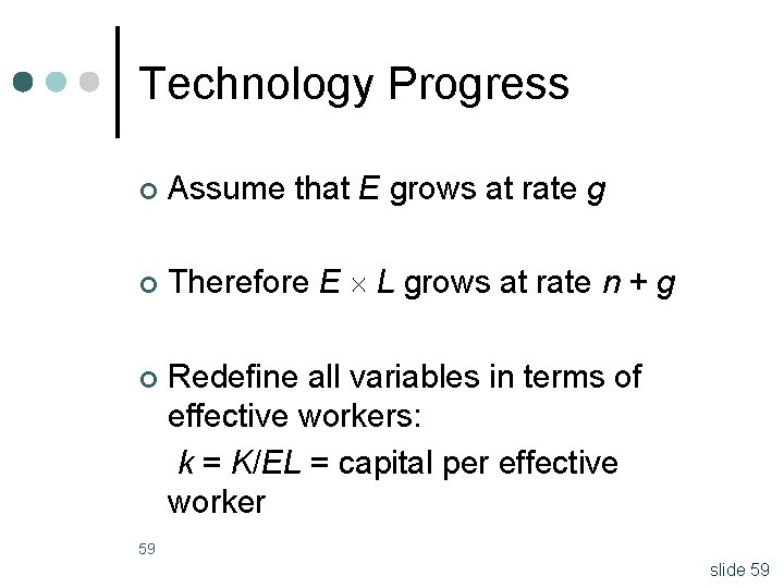
Technology Progress ¢ Assume that E grows at rate g ¢ Therefore E L grows at rate n + g ¢ Redefine all variables in terms of effective workers: k = K/EL = capital per effective worker 59 slide 59

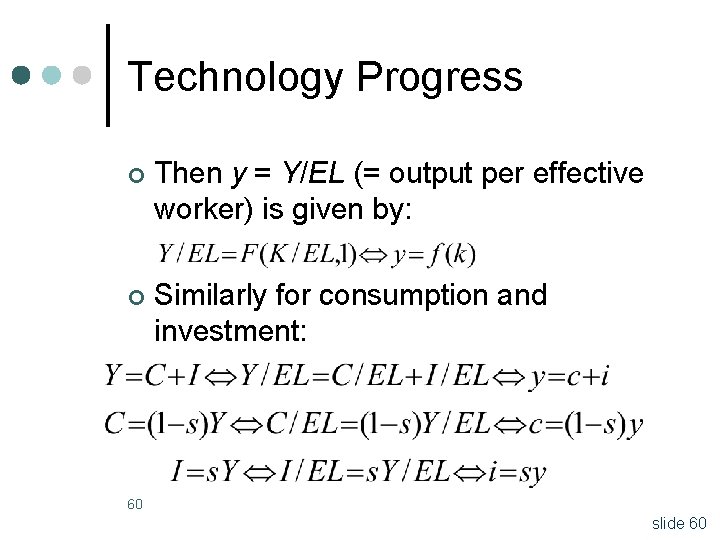
Technology Progress ¢ Then y = Y/EL (= output per effective worker) is given by: ¢ Similarly for consumption and investment: 60 slide 60

Technology Progress ¢ ¢ Therefore, the equations are the same as before The only change is in the law of motion for k. Capital per effective worker: l l l Increases with investment Decreases with physical depreciation Also decreases because there are more effective workers to share the existing capital (higher L and E) 61 slide 61

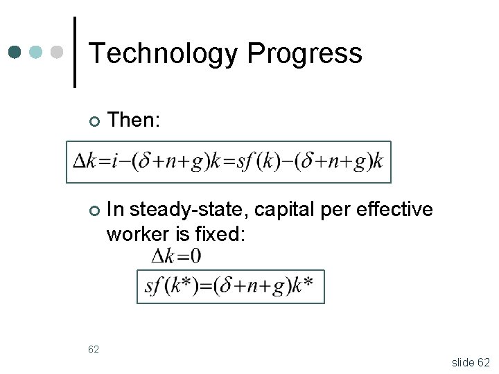
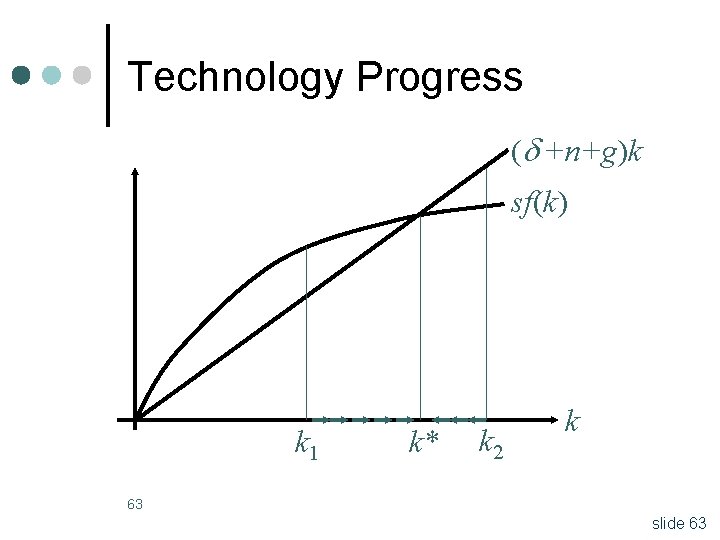
Technology Progress ¢ Then: ¢ In steady-state, capital per effective worker is fixed: 62 slide 62

Technology Progress ( +n+g)k sf(k) k 1 k* k 2 k 63 slide 63

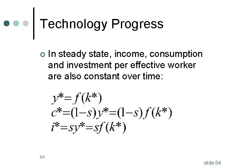
Technology Progress ¢ In steady state, income, consumption and investment per effective worker are also constant over time: 64 slide 64

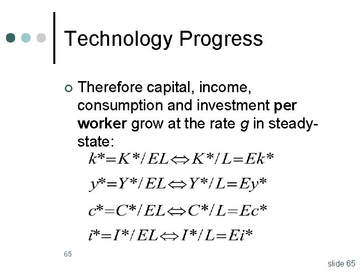
Technology Progress ¢ Therefore capital, income, consumption and investment per worker grow at the rate g in steadystate: 65 slide 65

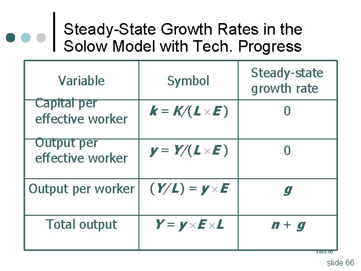
Steady-State Growth Rates in the Solow Model with Tech. Progress Variable Symbol Capital per effective worker Steady-state growth rate k = K/ (L E ) 0 Output per effective worker y = Y/ (L E ) 0 Output per worker (Y/ L ) = y E g Total output Y = y E L n+g slide 66

Technology Progress ¢ This follows since steady-state variables are constant and E is growing at the rate g ¢ Therefore, the inclusion of technology progress in the Solow model can generate sustained long-run growth 67 slide 67

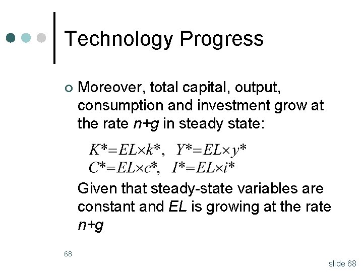
Technology Progress ¢ Moreover, total capital, output, consumption and investment grow at the rate n+g in steady state: Given that steady-state variables are constant and EL is growing at the rate n+g 68 slide 68

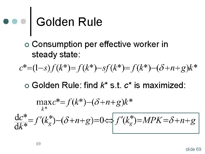
Golden Rule ¢ Consumption per effective worker in steady state: ¢ Golden Rule: find k* s. t. c* is maximized: 69 slide 69

Government Policies to raise the rate of productivity growth l l Improving infrastructure Would increased infrastructure spending increase productivity? • There might be reverse causation: Richer countries with higher productivity spend more on infrastructure, rather than vice versa • Infrastructure investments by government may be inefficient, since politics, not economic efficiency, is often the main determinant slide 70

Government Policies to raise the rate of productivity growth l l Building human capital • There’s a strong connection between productivity and human capital • Government can encourage human capital formation through educational policies, worker training and relocation programs, and health programs • Another form of human capital is entrepreneurial skill • Government could help by removing barriers like red tape Encouraging research and development • Government can encourage R and D through direct aid to research slide 71

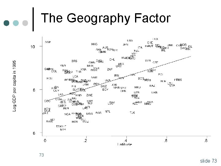
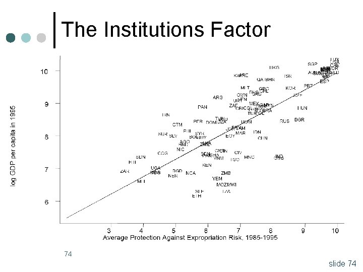
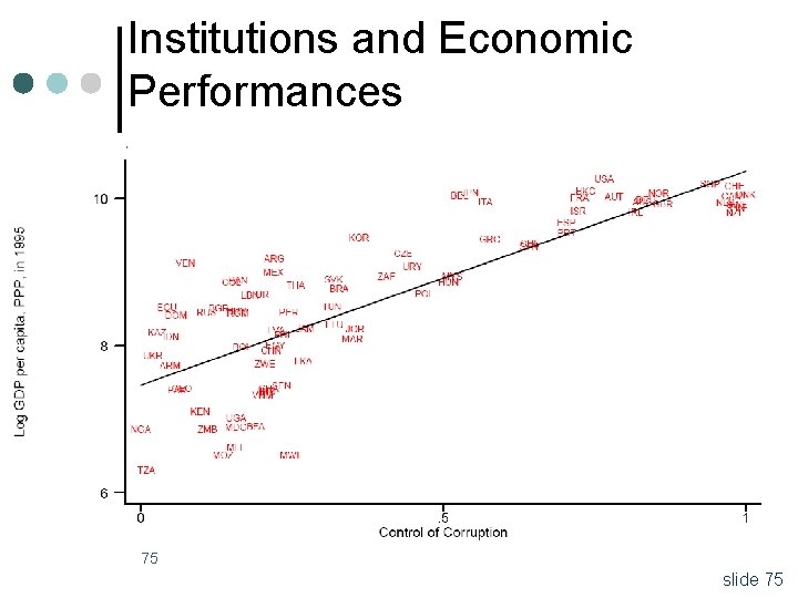
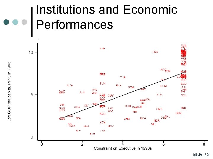
Why is technological breakthroughs progress so unequal across countries? ¢ What determined whether/when new technology adopted? Geography view: importance of ecology, climate, disease environment, geography, in short, factors outside human control. l Institutions view: importance of man-made factors; especially organization of society that provide incentives to individuals and firms. l History’s accidents: some countries are unlucky and trapped in underdevelopment. l 72 slide 72

The Geography Factor 73 slide 73

The Institutions Factor 74 slide 74

Institutions and Economic Performances 75 slide 75

Institutions and Economic Performances 76 slide 76

But institutions are complicated: identification problem ¢ Good institutions are correlated with many other good things. Theories about institutions are thus very difficult to test. ¢ The study of the causal role of institutions on economic growth is therefore complicated by concerns about endogeneity. ¢ For example, the United States is rich; it has good institutions; it has high levels of education; it has a common law heritage; it has a temperate climate. ¢ Good institutions are difficult to pin down precisely. We want to be very careful to disentangle different causal effects and isolate the effect of interest. 77 slide 77

But institutions are also endogenous Institutions could vary because underlying factors differ across countries: Geography, ecology, climate ¢ Montesquieu’s story: – Geography determines “human attitudes” – Human attitudes determine both economic performance and political system. – Institutions potentially influenced by the determinants of income ¢ 78 slide 78

Factor Prices ¢ So far, we solved the model without any reference to wages and rental rates (factor prices) ¢ We just focused on how income is generated, but not on how it is distributed ¢ Assume that a competitive firm hires capital and labor to generate output 79 slide 79

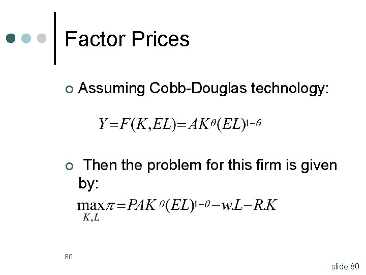
Factor Prices ¢ Assuming Cobb-Douglas technology: ¢ Then the problem for this firm is given by: 80 slide 80

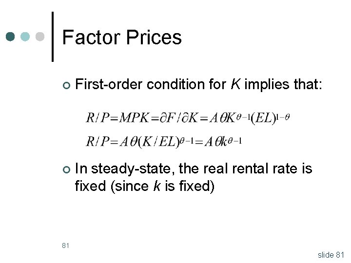
Factor Prices ¢ First-order condition for K implies that: ¢ In steady-state, the real rental rate is fixed (since k is fixed) 81 slide 81

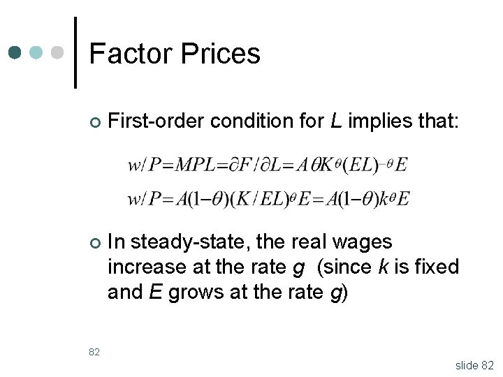
Factor Prices ¢ First-order condition for L implies that: ¢ In steady-state, the real wages increase at the rate g (since k is fixed and E grows at the rate g) 82 slide 82

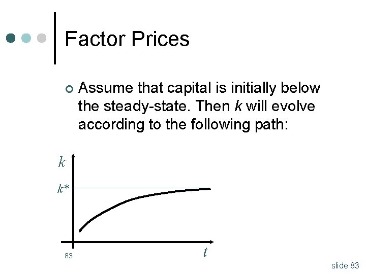
Factor Prices ¢ Assume that capital is initially below the steady-state. Then k will evolve according to the following path: k k* 83 t slide 83

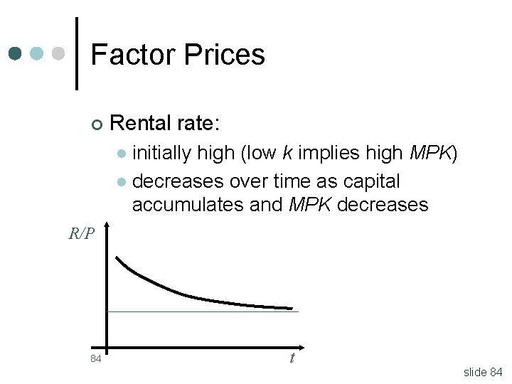
Factor Prices ¢ Rental rate: initially high (low k implies high MPK) l decreases over time as capital accumulates and MPK decreases l R/P 84 t slide 84

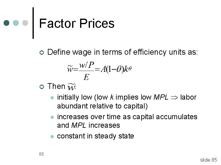
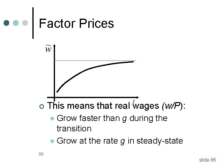
Factor Prices ¢ Define wage in terms of efficiency units as: ¢ Then l l l : initially low (low k implies low MPL labor abundant relative to capital) increases over time as capital accumulates and MPL increases constant in steady state 85 slide 85

Factor Prices ¢ t This means that real wages (w/P): Grow faster than g during the transition l Grow at the rate g in steady-state l 86 slide 86

Growth Accounting Want to be able to explain why and how countries grow ¢ There are many sources of growth ¢ First step is to decompose aggregate growth into its components: ¢ Growth in the labor force l Growth in capital l Growth in productivity l 87 slide 87

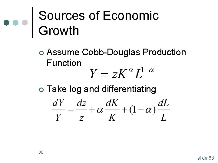
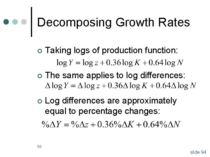
Sources of Economic Growth ¢ Assume Cobb-Douglas Production Function ¢ Take log and differentiating 88 slide 88

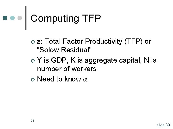
Computing TFP z: Total Factor Productivity (TFP) or “Solow Residual” ¢ Y is GDP, K is aggregate capital, N is number of workers ¢ Need to know α ¢ 89 slide 89

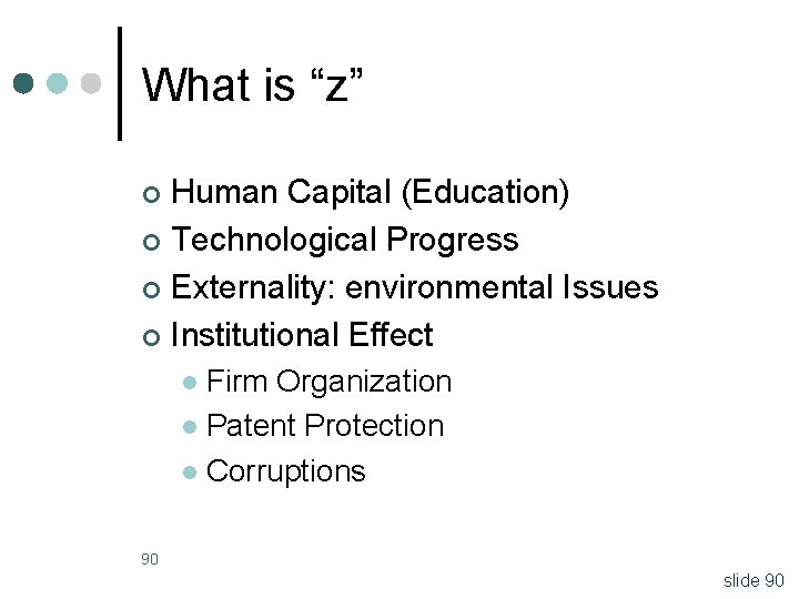
What is “z” Human Capital (Education) ¢ Technological Progress ¢ Externality: environmental Issues ¢ Institutional Effect ¢ Firm Organization l Patent Protection l Corruptions l 90 slide 90

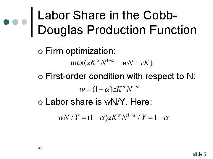
Labor Share in the Cobb. Douglas Production Function ¢ Firm optimization: ¢ First-order condition with respect to N: ¢ Labor share is w. N/Y. Here: 91 slide 91

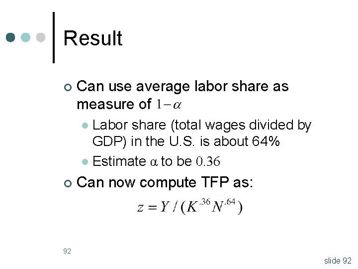
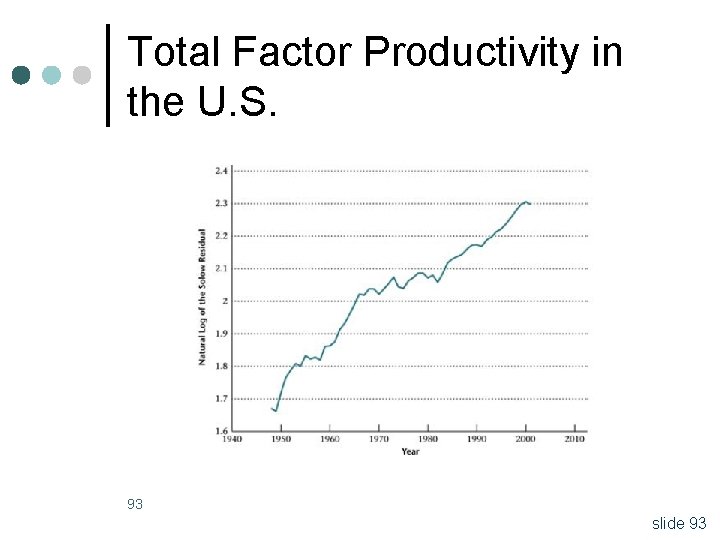
Result ¢ Can use average labor share as measure of Labor share (total wages divided by GDP) in the U. S. is about 64% l Estimate α to be 0. 36 l ¢ Can now compute TFP as: 92 slide 92

Total Factor Productivity in the U. S. 93 slide 93

Decomposing Growth Rates ¢ Taking logs of production function: ¢ The same applies to log differences: ¢ Log differences are approximately equal to percentage changes: 94 slide 94

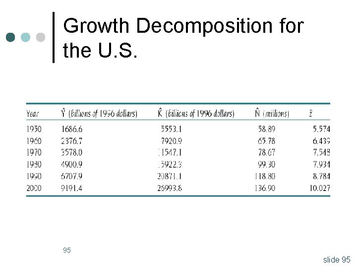
Growth Decomposition for the U. S. 95 slide 95

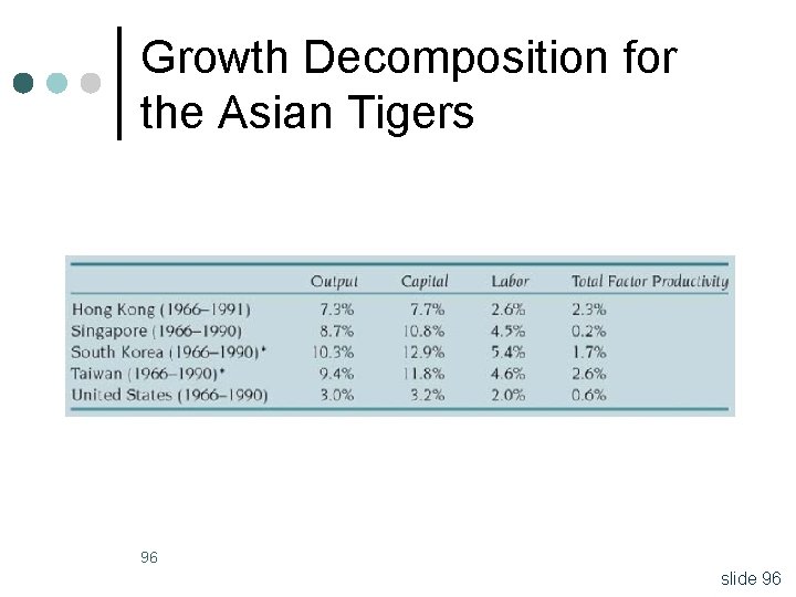
Growth Decomposition for the Asian Tigers 96 slide 96

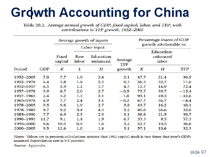
Growth Accounting for China slide 97

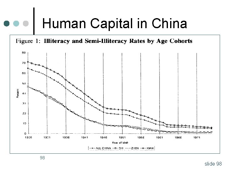
Human Capital in China 98 slide 98

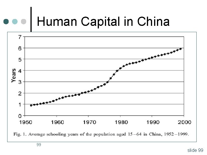
Human Capital in China 99 slide 99

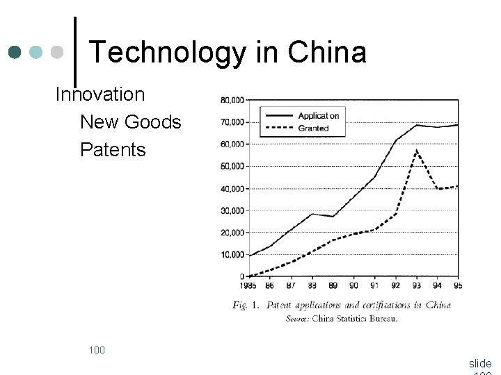
Technology in China Innovation New Goods Patents 100 slide

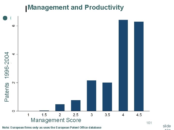
Patents 1996 -2004 Management and Productivity Management Score Note: European firms only as uses the European Patent Office database 101 slide

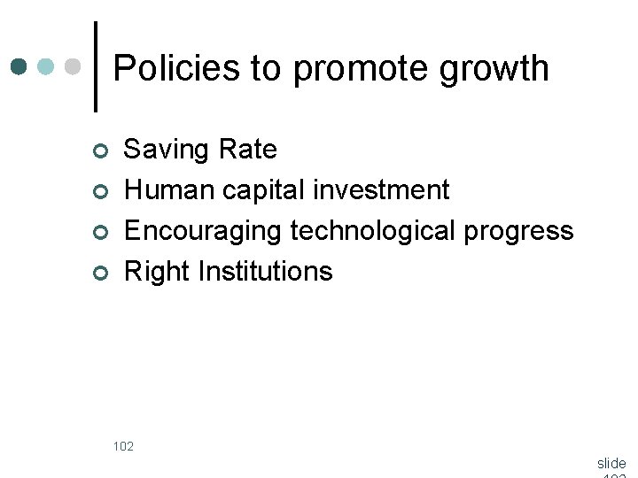
Policies to promote growth ¢ ¢ Saving Rate Human capital investment Encouraging technological progress Right Institutions 102 slide

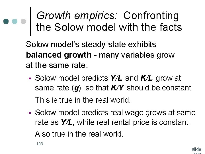
Growth empirics: Confronting the Solow model with the facts Solow model’s steady state exhibits balanced growth - many variables grow at the same rate. § Solow model predicts Y/L and K/L grow at same rate (g), so that K/Y should be constant. This is true in the real world. § Solow model predicts real wage grows at same rate as Y/L, while real rental price is constant. Also true in the real world. 103 slide

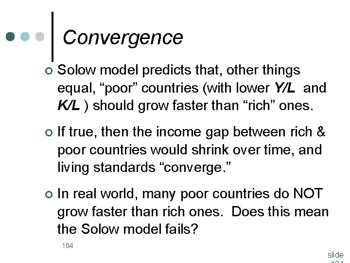
Convergence ¢ Solow model predicts that, other things equal, “poor” countries (with lower Y/L and K/L ) should grow faster than “rich” ones. ¢ If true, then the income gap between rich & poor countries would shrink over time, and living standards “converge. ” ¢ In real world, many poor countries do NOT grow faster than rich ones. Does this mean the Solow model fails? 104 slide

Convergence ¢ No, because “other things” aren’t equal. § In samples of countries with similar savings & pop. growth rates, income gaps shrink about 2%/year. § In larger samples, if one controls for differences in saving, population growth, and human capital, incomes converge by about 2%/year. 105 slide

Convergence ¢ What the Solow model really predicts is conditional convergence - countries converge to their own steady states, which are determined by saving, population growth, and education. And this prediction comes true in the real world. 106 slide