Lecture 12 Capacity Management and Planning continued Books

Lecture 12 Capacity Management and Planning (continued) Books • Introduction to Materials Management, Sixth Edition, J. R. Tony Arnold, P. E. , CFPIM, CIRM, Fleming College, Emeritus, Stephen N. Chapman, Ph. D. , CFPIM, North Carolina State University, Lloyd M. Clive, P. E. , CFPIM, Fleming College • Operations Management for Competitive Advantage, 11 th Edition, by Chase, Jacobs, and Aquilano, 2005, N. Y. : Mc. Graw-Hill/Irwin. • Operations Management, 11/E, Jay Heizer, Texas Lutheran University, Barry Render, Graduate School of Business, Rollins College, Prentice Hall

Objectives • • Managing Demand Tactics for managing demand Approaches to capacity expansion Breakeven analysis Decision tree and capacity expansion Net present value Capacity planning issues

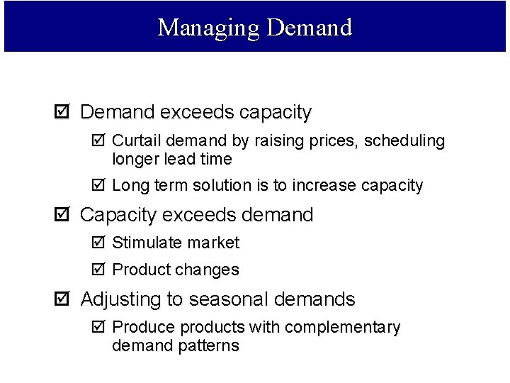
Managing Demand þ Demand exceeds capacity þ Curtail demand by raising prices, scheduling longer lead time þ Long term solution is to increase capacity þ Capacity exceeds demand þ Stimulate market þ Product changes þ Adjusting to seasonal demands þ Produce products with complementary demand patterns

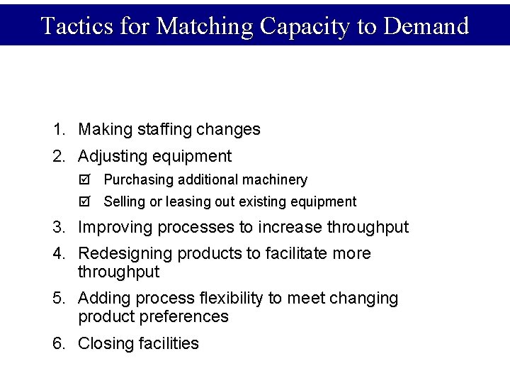
Tactics for Matching Capacity to Demand 1. Making staffing changes 2. Adjusting equipment þ Purchasing additional machinery þ Selling or leasing out existing equipment 3. Improving processes to increase throughput 4. Redesigning products to facilitate more throughput 5. Adding process flexibility to meet changing product preferences 6. Closing facilities

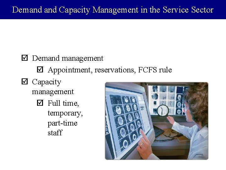
Demand Capacity Management in the Service Sector þ Demand management þ Appointment, reservations, FCFS rule þ Capacity management þ Full time, temporary, part-time staff

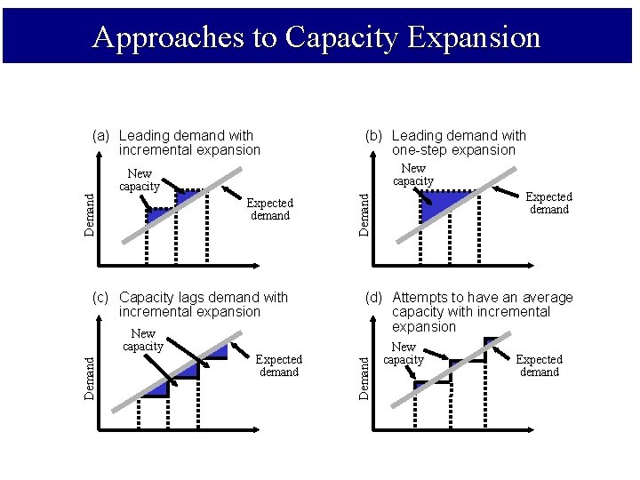
Approaches to Capacity Expansion New capacity Expected demand (c) Capacity lags demand with incremental expansion Demand Expected demand Demand New capacity (b) Leading demand with one-step expansion (d) Attempts to have an average capacity with incremental expansion Demand (a) Leading demand with incremental expansion New capacity Expected demand

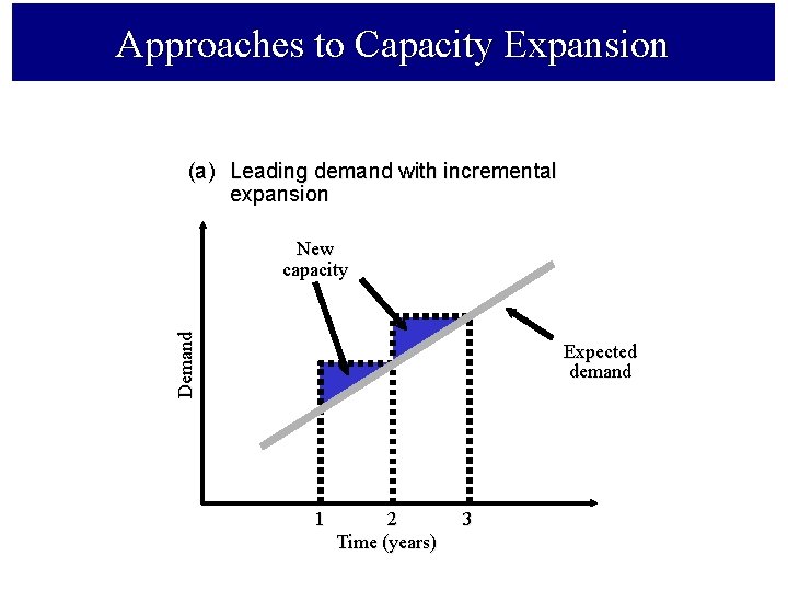
Approaches to Capacity Expansion (a) Leading demand with incremental expansion Demand New capacity Expected demand 1 2 Time (years) 3

Approaches to Capacity Expansion (b) Leading demand with one-step expansion New capacity Demand Expected demand 1 2 Time (years) 3

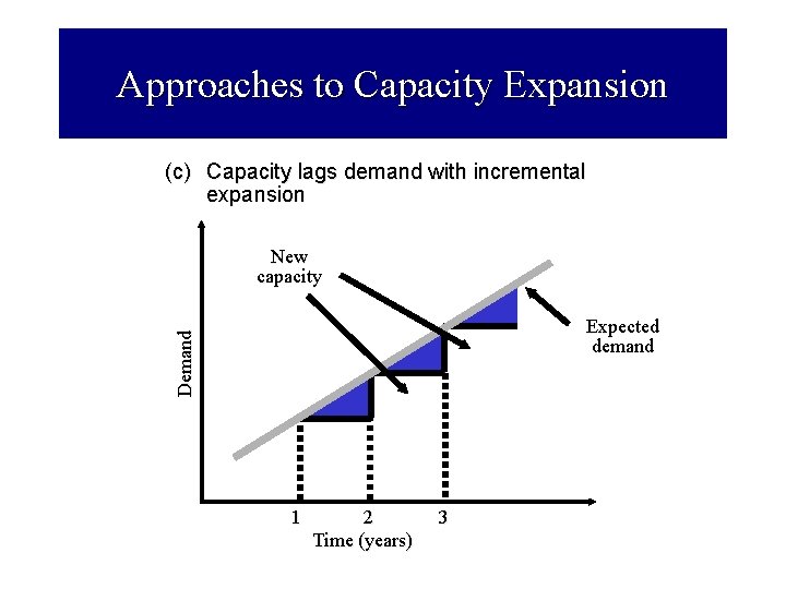
Approaches to Capacity Expansion (c) Capacity lags demand with incremental expansion New capacity Demand Expected demand 1 2 Time (years) 3

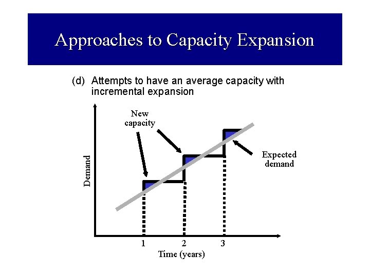
Approaches to Capacity Expansion (d) Attempts to have an average capacity with incremental expansion New capacity Demand Expected demand 1 2 Time (years) 3

Break-Even Analysis þ Technique for evaluating process and equipment alternatives þ Objective is to find the point in dollars and units at which cost equals revenue þ Requires estimation of fixed costs, variable costs, and revenue

Break-Even Analysis þ Fixed costs are costs that continue even if no units are produced þ Depreciation, taxes, debt, mortgage payments þ Variable costs are costs that vary with the volume of units produced þ Labor, materials, portion of utilities þ Contribution is the difference between selling price and variable cost

Break-Even Analysis Assumptions þ Costs and revenue are linear functions þ Generally not the case in the real world þ We actually know these costs þ Very difficult to accomplish þ There is no time value of money

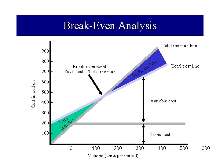
Break-Even Analysis – Total revenue line 900 – 800 – Cost in dollars 700 – Break-even point Total cost = Total revenue d rri o it c or Total cost line f Pro 600 – 500 – Variable cost 400 – 300 – 200 – 100 – – ss r Lo rido r co Fixed cost | 0 | | | 100 200 300 Volume (units period) | | | 400 500 600

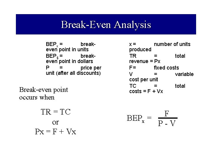
Break-Even Analysis BEPx = breakeven point in units BEP$ = breakeven point in dollars P = price per unit (after all discounts) Break-even point occurs when TR = TC or Px = F + Vx x= number of units produced TR = total revenue = Px F= fixed costs V = variable cost per unit TC = total costs = F + Vx F BEPx = P-V

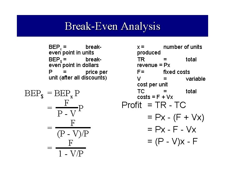
Break-Even Analysis BEPx = breakeven point in units BEP$ = breakeven point in dollars P = price per unit (after all discounts) BEP$ = BEPx P F = P P-V F = (P - V)/P F = 1 - V/P x= number of units produced TR = total revenue = Px F= fixed costs V = variable cost per unit TC = total costs = F + Vx Profit = TR - TC = Px - (F + Vx) = Px - F - Vx = (P - V )x - F

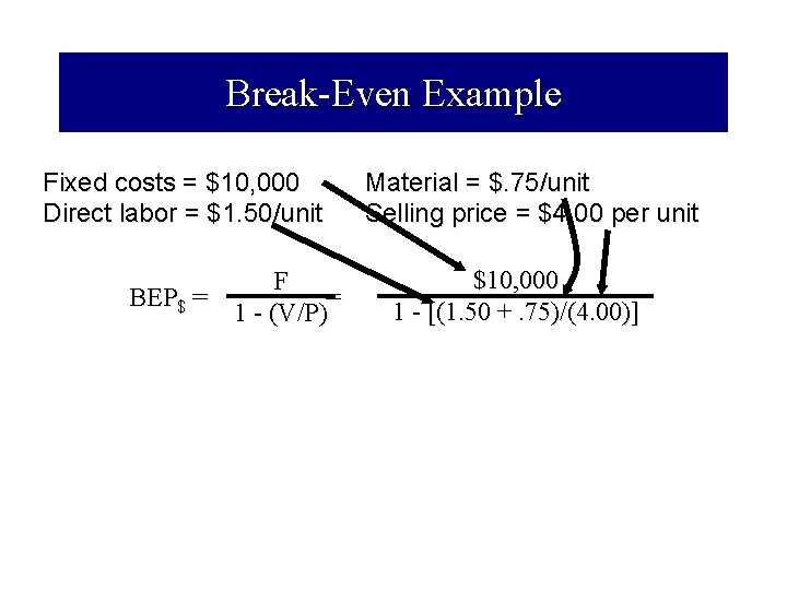
Break-Even Example Fixed costs = $10, 000 Direct labor = $1. 50/unit F BEP$ = = 1 - (V/P) Material = $. 75/unit Selling price = $4. 00 per unit $10, 000 1 - [(1. 50 +. 75)/(4. 00)]

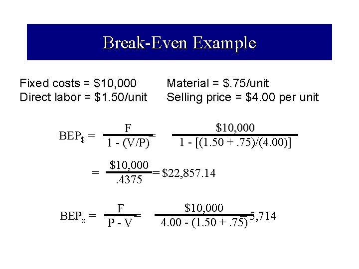
Break-Even Example Fixed costs = $10, 000 Direct labor = $1. 50/unit F BEP$ = = 1 - (V/P) Material = $. 75/unit Selling price = $4. 00 per unit $10, 000 1 - [(1. 50 +. 75)/(4. 00)] $10, 000 = = $22, 857. 14. 4375 F BEPx = = P-V $10, 000 = 5, 714 4. 00 - (1. 50 +. 75)

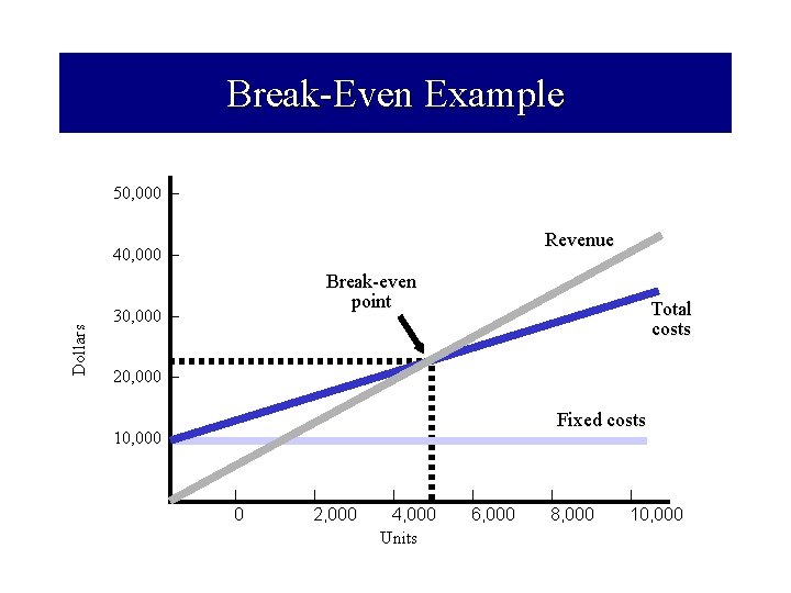
Break-Even Example 50, 000 – Revenue Dollars 40, 000 – Break-even point 30, 000 – Total costs 20, 000 – Fixed costs 10, 000 – – | | 0 2, 000 | 4, 000 Units | | | 6, 000 8, 000 10, 000

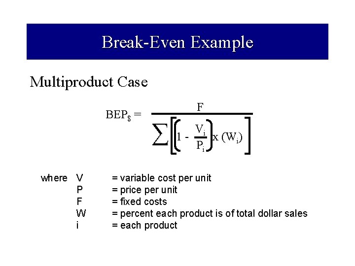
Break-Even Example Multiproduct Case BEP$ = where V P F W i F ∑ Vi 1 x (W i ) Pi = variable cost per unit = price per unit = fixed costs = percent each product is of total dollar sales = each product

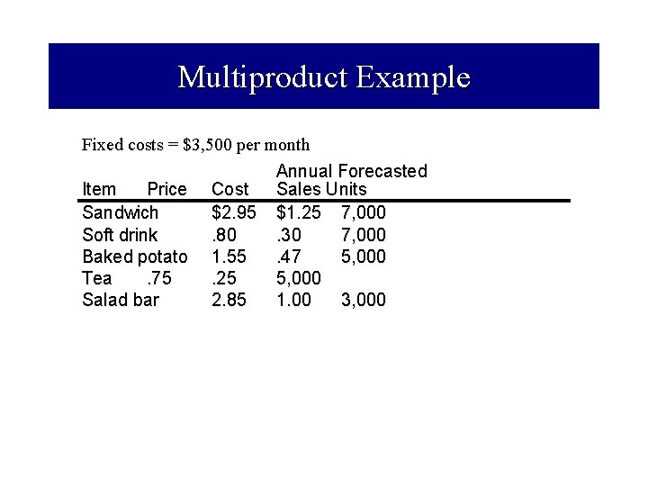
Multiproduct Example Fixed costs = $3, 500 per month Annual Forecasted Item Price Cost Sales Units Sandwich $2. 95 $1. 25 7, 000 Soft drink. 80. 30 7, 000 Baked potato 1. 55. 47 5, 000 Tea. 75. 25 5, 000 Salad bar 2. 85 1. 00 3, 000

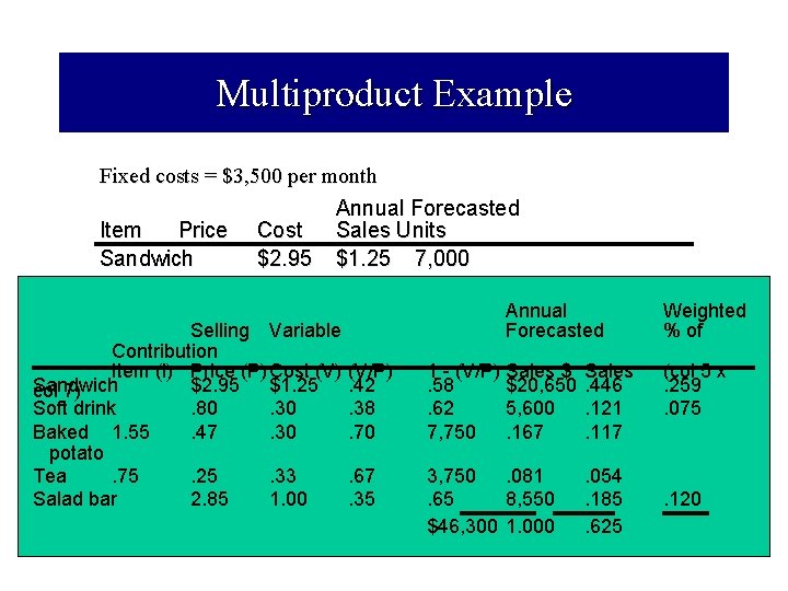
Multiproduct Example Fixed costs = $3, 500 per month Annual Forecasted Item Price Cost Sales Units Sandwich $2. 95 $1. 25 7, 000 Soft drink. 80. 30 7, 000 Annual Baked potato 1. 55. 47 5, 000 Selling. 25 Variable 5, 000 Forecasted Tea. 75 Contribution Salad bar. Price (P)2. 85 Item (i) Cost (V)1. 00 (V/P) 3, 000 1 - (V/P) Sales $ Sales Sandwich col 7) Soft drink Baked 1. 55 potato Tea. 75 Salad bar $2. 95. 80. 47 $1. 25. 30 . 42. 38. 70 . 58. 62 7, 750 $20, 650. 446 5, 600. 121. 167. 117 . 25 2. 85 . 33 1. 00 . 67. 35 3, 750. 081. 65 8, 550 $46, 300 1. 000 . 054. 185. 625 Weighted % of (col 5 x. 259. 075 . 120

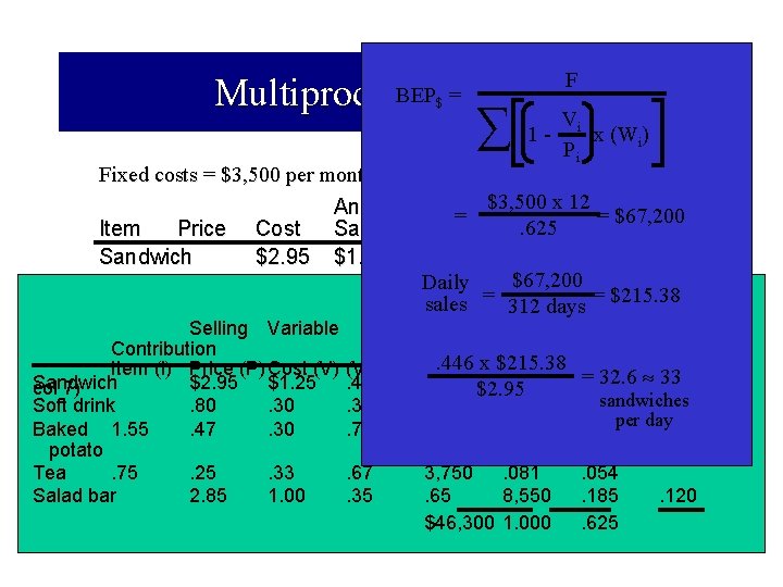
F BEPExample = Multiproduct V $ ∑ 1 - i Pi x (Wi) Fixed costs = $3, 500 per month $3, 500 x 12 Annual Forecasted = = $67, 200. 625 Item Price Cost Sales Units Sandwich $2. 95 $1. 25 7, 000 $67, 200 Daily Soft drink. 80. 30 7, 000 = = $215. 38 sales 312 days Annual Weighted Baked potato 1. 55. 47 5, 000 Selling. 25 Variable 5, 000 Forecasted % of Tea. 75 Contribution x $215. 38 Salad bar. Price (P)2. 85 Item (i) Cost (V)1. 00 (V/P) 3, 000 1. 446 - (V/P) Sales $ Sales (col = 32. 6 . 259 33 5 x Sandwich $2. 95 $1. 25. 42. 58 $20, 650. 446 col 7) $2. 95 Soft drink Baked 1. 55 potato Tea. 75 Salad bar . 80. 47 . 30 . 38. 70 . 62 7, 750 5, 600. 167 . 25 2. 85 . 33 1. 00 . 67. 35 3, 750. 081. 65 8, 550 $46, 300 1. 000 sandwiches. 121. 075. 117 per day. 054. 185. 625 . 120

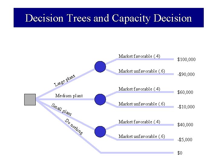
Decision Trees and Capacity Decision Market favorable (. 4) t lan p ge r a L Market unfavorable (. 6) Market favorable (. 4) Medium plant Sm all pla nt Do no thi ng Market unfavorable (. 6) Market favorable (. 4) Market unfavorable (. 6) $100, 000 -$90, 000 $60, 000 -$10, 000 $40, 000 -$5, 000 $0

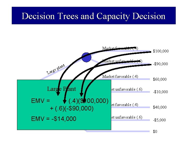
Decision Trees and Capacity Decision Market favorable (. 4) t lan p ge r a L Market unfavorable (. 6) Market favorable (. 4) Medium plant Market unfavorable (. 6) Large Plant Sm all pla nt EMV = Do (. 4)($100, 000) Market favorable (. 4) no thi + (. 6)(-$90, 000) ng Market unfavorable (. 6) EMV = -$14, 000 $100, 000 -$90, 000 $60, 000 -$10, 000 $40, 000 -$5, 000 $0

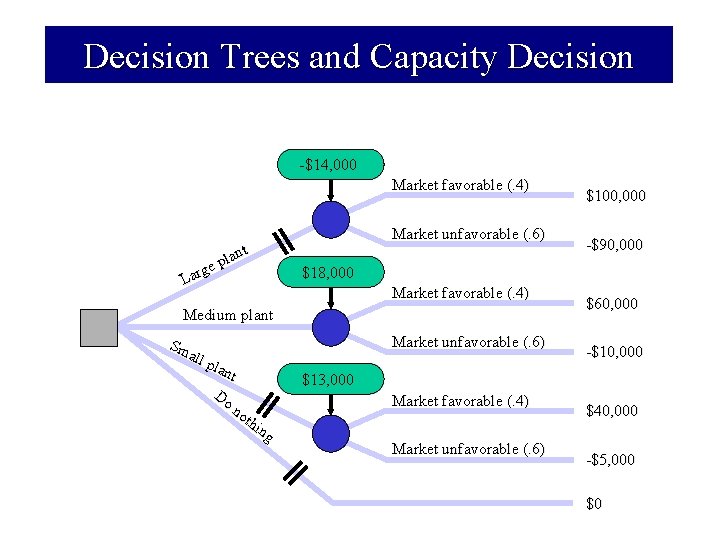
Decision Trees and Capacity Decision -$14, 000 Market favorable (. 4) t lan p ge r a L Market unfavorable (. 6) -$90, 000 $18, 000 Market favorable (. 4) Medium plant Sm all pla nt Do no thi ng $100, 000 Market unfavorable (. 6) $60, 000 -$10, 000 $13, 000 Market favorable (. 4) Market unfavorable (. 6) $40, 000 -$5, 000 $0

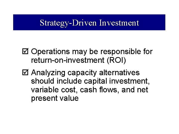
Strategy-Driven Investment þ Operations may be responsible for return-on-investment (ROI) þ Analyzing capacity alternatives should include capital investment, variable cost, cash flows, and net present value

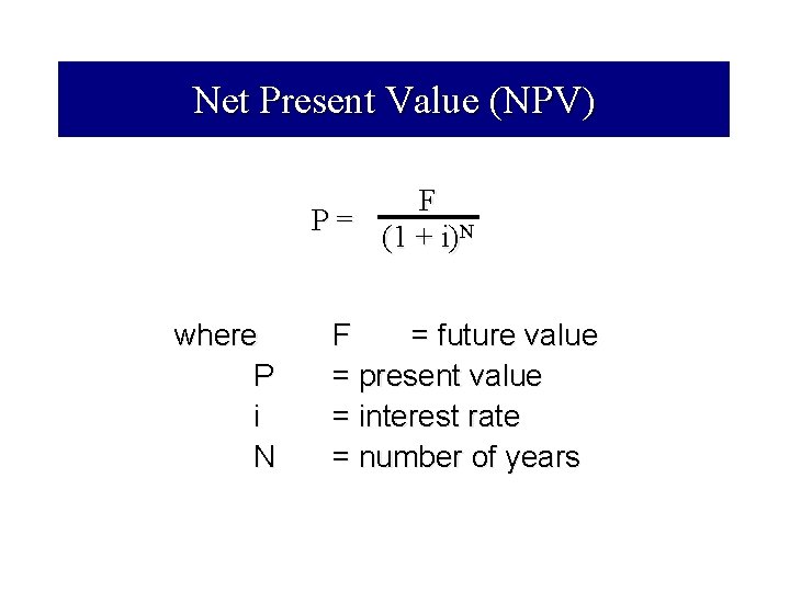
Net Present Value (NPV) F P= (1 + i)N where P i N F = future value = present value = interest rate = number of years

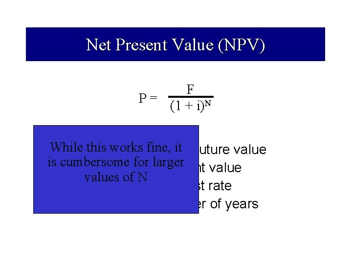
Net Present Value (NPV) F P= (1 + i)N Whilewhere this works fine, F it = future value is cumbersome P for=larger present values of N i = interest rate N = number of years

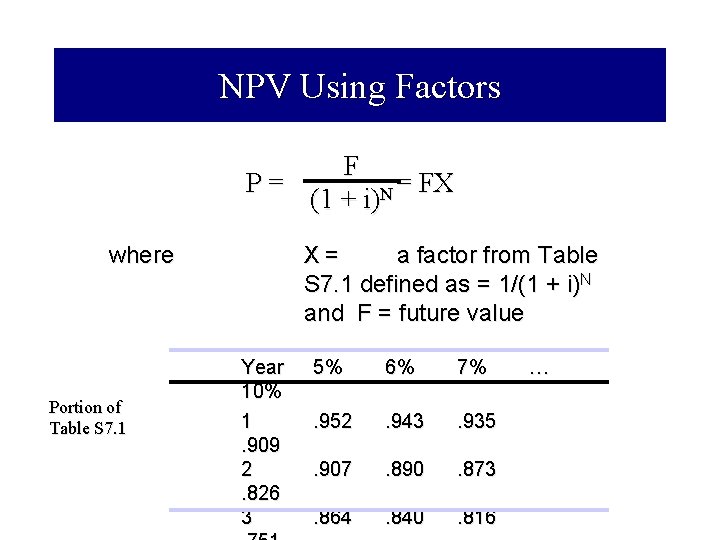
NPV Using Factors F P= = FX N (1 + i) where Portion of Table S 7. 1 X= a factor from Table S 7. 1 defined as = 1/(1 + i)N and F = future value Year 10% 1. 909 2. 826 3 5% 6% 7% . 952 . 943 . 935 . 907 . 890 . 873 . 864 . 840 . 816 …

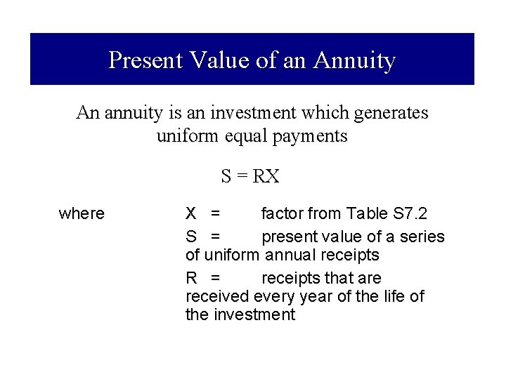
Present Value of an Annuity An annuity is an investment which generates uniform equal payments S = RX where X = factor from Table S 7. 2 S = present value of a series of uniform annual receipts R = receipts that are received every year of the life of the investment

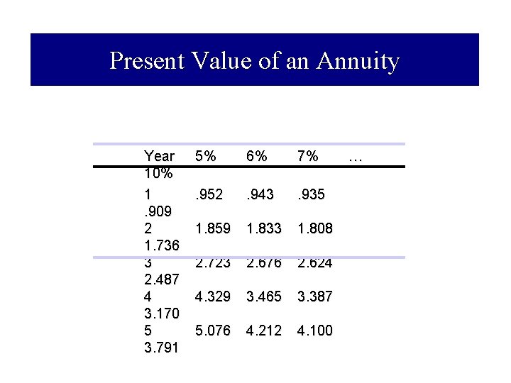
Present Value of an Annuity Year 10% 1. 909 2 1. 736 3 2. 487 4 3. 170 5 3. 791 5% 6% 7% . 952 . 943 . 935 1. 859 1. 833 1. 808 2. 723 2. 676 2. 624 4. 329 3. 465 3. 387 5. 076 4. 212 4. 100 …

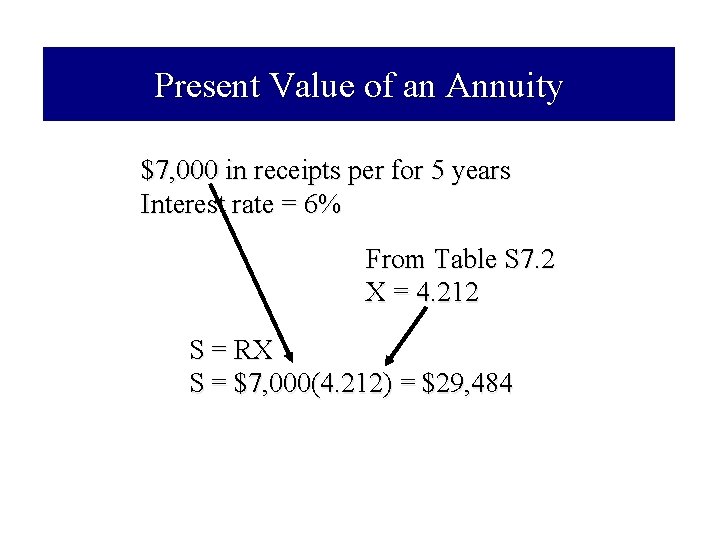
Present Value of an Annuity $7, 000 in receipts per for 5 years Interest rate = 6% From Table S 7. 2 X = 4. 212 S = RX S = $7, 000(4. 212) = $29, 484

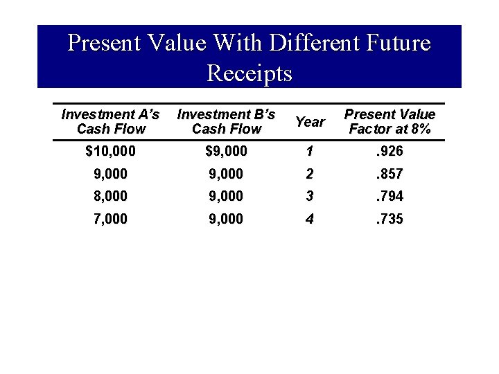
Present Value With Different Future Receipts Investment A’s Cash Flow Investment B’s Cash Flow Year Present Value Factor at 8% $10, 000 $9, 000 1 . 926 9, 000 2 . 857 8, 000 9, 000 3 . 794 7, 000 9, 000 4 . 735

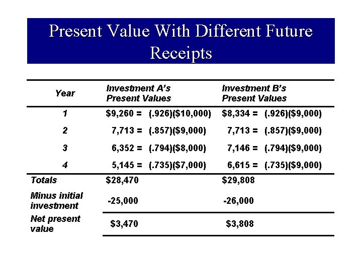
Present Value With Different Future Receipts Investment A’s Present Values Investment B’s Present Values 1 $9, 260 = (. 926)($10, 000) $8, 334 = (. 926)($9, 000) 2 7, 713 = (. 857)($9, 000) 3 6, 352 = (. 794)($8, 000) 7, 146 = (. 794)($9, 000) 4 5, 145 = (. 735)($7, 000) 6, 615 = (. 735)($9, 000) Year Totals Minus initial investment Net present value $28, 470 $29, 808 -25, 000 -26, 000 $3, 470 $3, 808

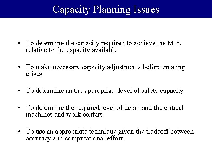
Capacity Planning Issues • To determine the capacity required to achieve the MPS relative to the capacity available • To make necessary capacity adjustments before creating crises • To determine an the appropriate level of safety capacity • To determine the required level of detail and the critical machines and work centers • To use an appropriate technique given the tradeoff between accuracy and computational effort

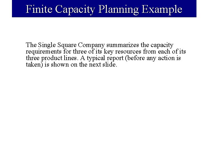
Finite Capacity Planning Example The Single Square Company summarizes the capacity requirements for three of its key resources from each of its three product lines. A typical report (before any action is taken) is shown on the next slide.

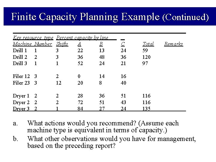
Finite Capacity Planning Example (Continued) Key resource type Machine Number Drill 1 1 Drill 2 2 Drill 3 1 Percent capacity by line Shifts A B 3 22 13 3 36 48 1 52 24 C 24 36 21 Filer 12 3 Filer 23 3 2 12 0 20 14 8 16 40 Dryer 1 2 Dryer 2 2 Dryer 3 2 2 2 1 28 72 84 36 51 27 51 43 24 a. b. Total 59 120 97 Remarks 116 135 What actions would you recommend? (Assume each machine type is equivalent in terms of capacity. ) What other observations would you have for management, based on the preceding report?

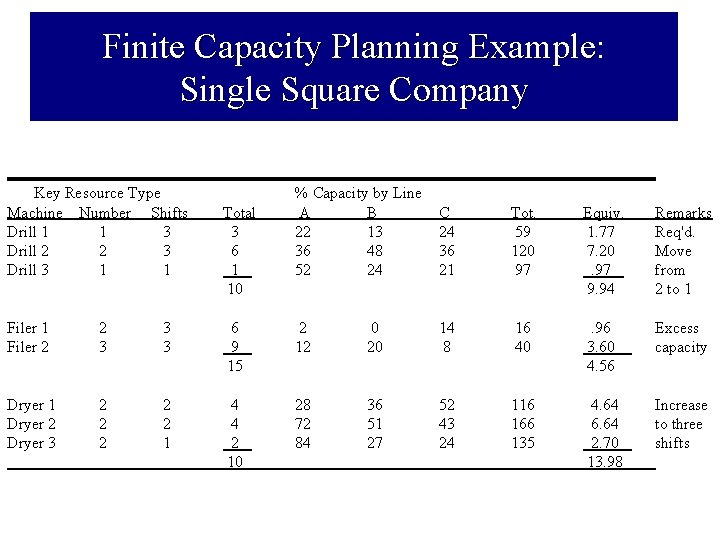
Finite Capacity Planning Example: Single Square Company Key Resource Type Machine Number Shifts Drill 1 1 3 Drill 2 2 3 Drill 3 1 1 Total 3 6 1 10 % Capacity by Line A B 22 13 36 48 52 24 C 24 36 21 Tot. 59 120 97 Equiv. 1. 77 7. 20. 97 9. 94 Remarks Req'd. Move from 2 to 1 Filer 2 2 3 3 3 6 9 15 2 12 0 20 14 8 16 40 . 96 3. 60 _ 4. 56 Excess capacity Dryer 1 Dryer 2 Dryer 3 2 2 2 1 4 4 2 10 28 72 84 36 51 27 52 43 24 116 166 135 4. 64 6. 64 2. 70 13. 98 Increase to three shifts

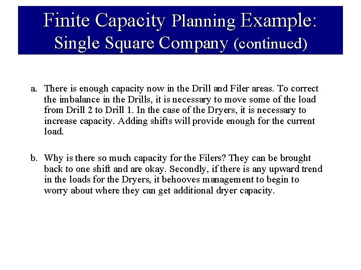
Finite Capacity Planning Example: Single Square Company (continued) a. There is enough capacity now in the Drill and Filer areas. To correct the imbalance in the Drills, it is necessary to move some of the load from Drill 2 to Drill 1. In the case of the Dryers, it is necessary to increase capacity. Adding shifts will provide enough for the current load. b. Why is there so much capacity for the Filers? They can be brought back to one shift and are okay. Secondly, if there is any upward trend in the loads for the Dryers, it behooves management to begin to worry about where they can get additional dryer capacity.

Twin Disc Capacity Bill Report 41

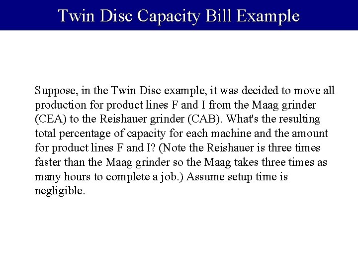
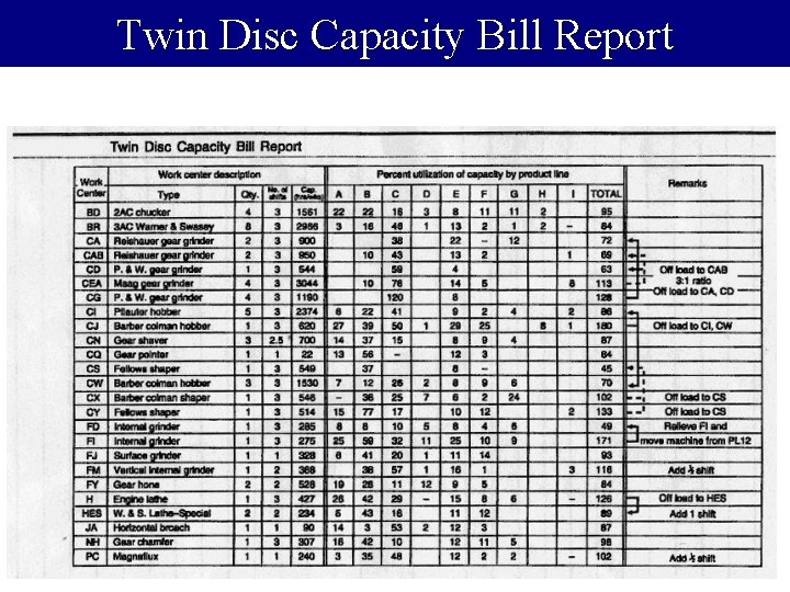
Twin Disc Capacity Bill Example Suppose, in the Twin Disc example, it was decided to move all production for product lines F and I from the Maag grinder (CEA) to the Reishauer grinder (CAB). What's the resulting total percentage of capacity for each machine and the amount for product lines F and I? (Note the Reishauer is three times faster than the Maag grinder so the Maag takes three times as many hours to complete a job. ) Assume setup time is negligible.

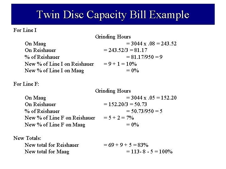
Twin Disc Capacity Bill Example For Line I Grinding Hours On Maag = 3044 x. 08 = 243. 52 On Reishauer = 243. 52/3 = 81. 17 % of Reishauer = 81. 17/950 = 9 New % of Line I on Reishauer = 9 + 1 = 10% New % of Line I on Maag = 0% For Line F: Grinding Hours On Maag = 3044 x. 05 = 152. 20 On Reishauer = 152. 20/3 = 50. 73 % of Reishauer = 50. 73/950 = 5 New % of Line F on Reishauer = 5 + 2 = 7% New % of Line F on Maag = 0% New Totals: New total for Reishauer New total for Maag = 69 + 5 = 83% = 113 - 8 - 5 = 100%

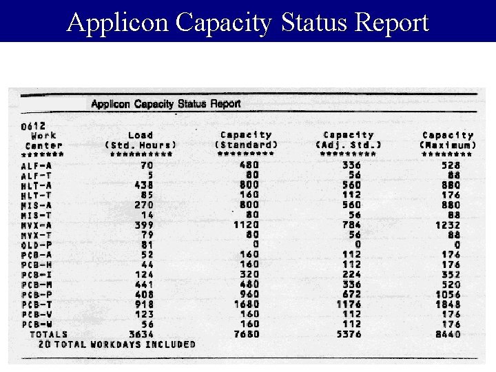
Applicon Capacity Status Report 44

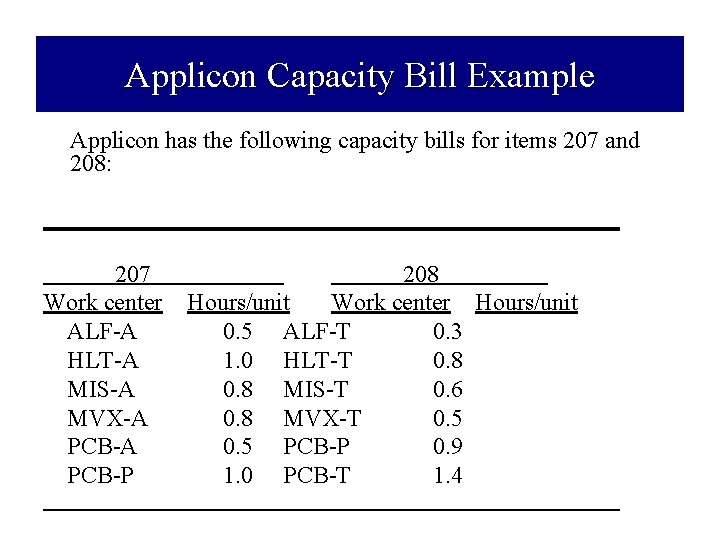
Applicon Capacity Bill Example Applicon has the following capacity bills for items 207 and 208: 207 Work center ALF-A HLT-A MIS-A MVX-A PCB-P 208 Hours/unit Work center Hours/unit 0. 5 ALF-T 0. 3 1. 0 HLT-T 0. 8 MIS-T 0. 6 0. 8 MVX-T 0. 5 PCB-P 0. 9 1. 0 PCB-T 1. 4

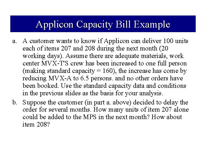
Applicon Capacity Bill Example a. A customer wants to know if Applicon can deliver 100 units each of items 207 and 208 during the next month (20 working days). Assume there adequate materials, work center MVX-T'S crew has been increased to one full person (making standard capacity = 160), the increase has come by reducing MVX-A to 6. 5 persons. and no other orders have been booked. Use the standard capacity data and conditions in the previous slides as the basis for your analysis. b. Suppose the customer (in part a. above) decided to delay the order for several months. How many units of item 207 alone could be added to the MPS in the next month? How about item 208?

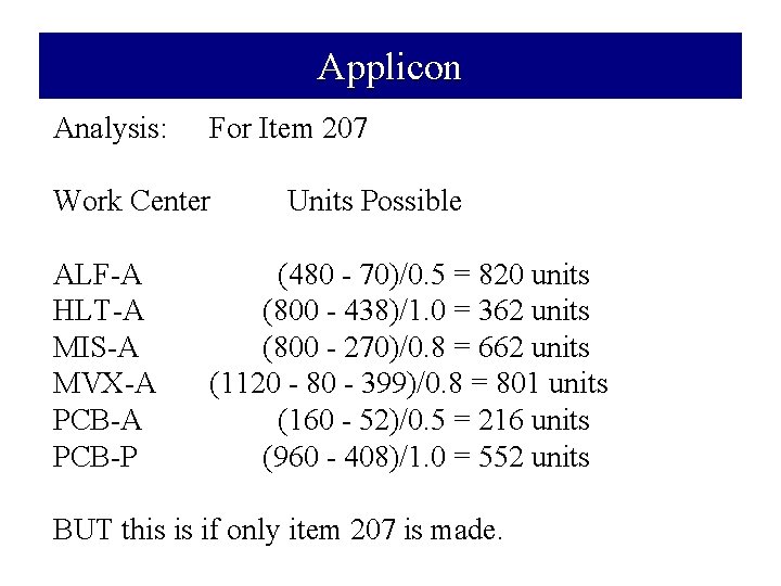
Applicon Analysis: For Item 207 Work Center ALF-A HLT-A MIS-A MVX-A PCB-P Units Possible (480 - 70)/0. 5 = 820 units (800 - 438)/1. 0 = 362 units (800 - 270)/0. 8 = 662 units (1120 - 80 - 399)/0. 8 = 801 units (160 - 52)/0. 5 = 216 units (960 - 408)/1. 0 = 552 units BUT this is if only item 207 is made.

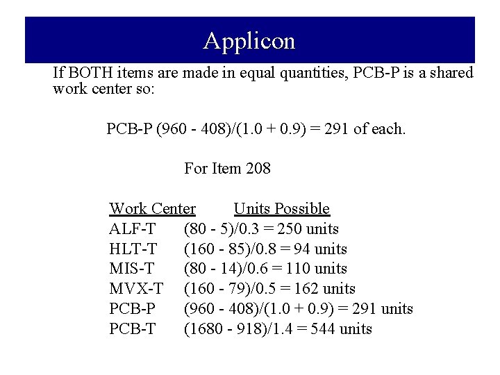
Applicon If BOTH items are made in equal quantities, PCB-P is a shared work center so: PCB-P (960 - 408)/(1. 0 + 0. 9) = 291 of each. For Item 208 Work Center Units Possible ALF-T (80 - 5)/0. 3 = 250 units HLT-T (160 - 85)/0. 8 = 94 units MIS-T (80 - 14)/0. 6 = 110 units MVX-T (160 - 79)/0. 5 = 162 units PCB-P (960 - 408)/(1. 0 + 0. 9) = 291 units PCB-T (1680 - 918)/1. 4 = 544 units

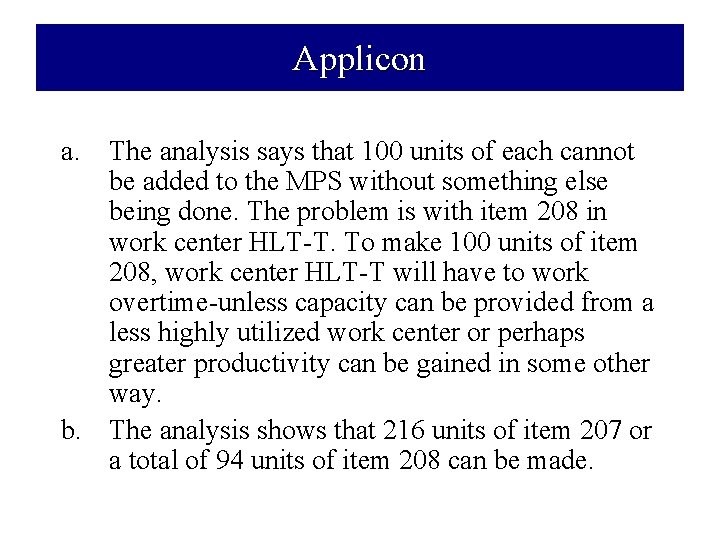
Applicon a. The analysis says that 100 units of each cannot be added to the MPS without something else being done. The problem is with item 208 in work center HLT-T. To make 100 units of item 208, work center HLT-T will have to work overtime-unless capacity can be provided from a less highly utilized work center or perhaps greater productivity can be gained in some other way. b. The analysis shows that 216 units of item 207 or a total of 94 units of item 208 can be made.

Concluding Principles • Capacity plans must be developed concurrently with material plans if the material plans are to be realized. • The capacity measure should reflect realizable output from the key resources. • It's not always capacity that should change when capacity availability doesn't equal need. • Capacity not only must be planned, but use of that capacity must also be monitored and controlled. • Capacity planning techniques can be applied to selected key resources (which need not correspond to production work centers).

Concluding Principles • The particular capacity planning technique(s) chosen must match the level of detail and actual company circumstances to permit making effective management decisions. • The more detail in the capacity planning system, the more data and data base maintenance are required. • The better the resource and production planning process, the less difficult the capacity planning process. • The better the shop-floor system, the less short-term capacity planning is required. • Capacity planning can be simplified in a JIT environment.

End of Lecture 12