Lecture 11 Principles of Mass Balance Simple Box

Lecture 11 Principles of Mass Balance Simple Box Models The modern view about what controls the composition of sea water.

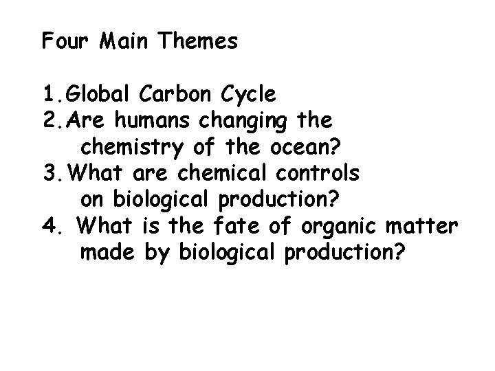
Four Main Themes 1. Global Carbon Cycle 2. Are humans changing the chemistry of the ocean? 3. What are chemical controls on biological production? 4. What is the fate of organic matter made by biological production?

Example: Global Carbon Cycle CO 2, atm = 590/130 = 4. 5 y C, biota = 3/50 = 0. 06 y C, export = 3/11 = 0. 29 y export/tbiota = 0. 27/0. 06 = 4. 5 times recycled No red export!

Two main types of models used in chemical oceanography. -Box (or reservoir) Models -Continuous Transport-reaction Models In both cases: Change in Mass with = Time Sum of Inputs - Sum of Outputs

At steady state the dissolved concentration (Mi) does not change with time: (d. M/dt)ocn = Sd. Mi / dt = 0 Sum of sources must equal sum of sinks at steady state

Box Models How would you verify that this 1 -Box Ocean is at steady state?

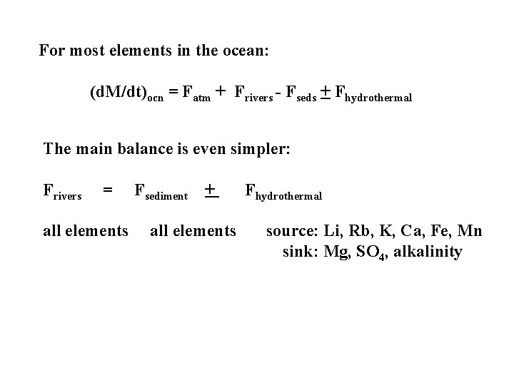
For most elements in the ocean: (d. M/dt)ocn = Fatm + Frivers - Fseds + Fhydrothermal The main balance is even simpler: Frivers = all elements Fsediment + all elements Fhydrothermal source: Li, Rb, K, Ca, Fe, Mn sink: Mg, SO 4, alkalinity

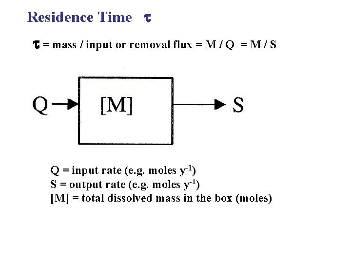
Residence Time = mass / input or removal flux = M / Q =M/S Q = input rate (e. g. moles y-1) S = output rate (e. g. moles y-1) [M] = total dissolved mass in the box (moles)

d[M] / dt = Q – S input = Q = Zeroth Order flux (e. g. river input) not proportional to how much is in the ocean sink = S = many are First Order (e. g. Radioactive decay, plankton uptake, adsorption by particles) If inflow equals outflow Q=S then d[M] / dt = 0 or steady state

First order removal is proportional to how much is there. S = k [M] where k (sometimes ) is the first order removal rate constant (t-1) and [M] is the total mass. Then: d[M] / dt = Q – k [M] at steady state when d[M] / dt = 0 [M] / Q = 1/k = and [M] = Q / k inverse relationship Q = k[M]

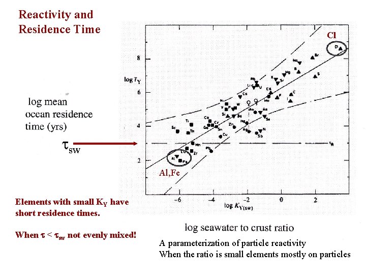
Reactivity and Residence Time Cl sw Al, Fe Elements with small KY have short residence times. When < sw not evenly mixed! A parameterization of particle reactivity When the ratio is small elements mostly on particles

Dynamic Box Models If the source (Q) and sink (S) rates are not constant with time or they may have been constant and suddenly change. Examples: Glacial/Interglacial; Anthropogenic Inputs to Ocean Assume that the initial amount of M at t = 0 is Mo. The initial mass balance equation is: d. M/dt = Qo – So = Qo – k Mo The input increases to a new value Q 1. The new balance at the new steady state is: d. M/dt = Q 1 – k M and the solution for the approach to the new equilibrium state is: M(t) = M 1 – (M 1 – Mo) exp ( -k t ) M increases from Mo to the new value of M 1 (= Q 1 / k) with a response time of k-1 or

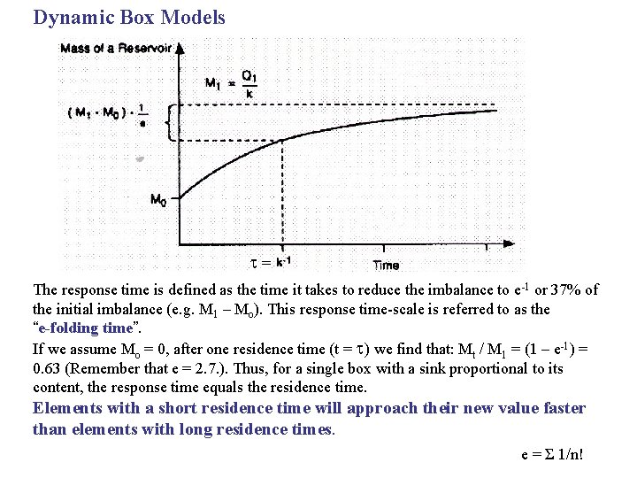
Dynamic Box Models = The response time is defined as the time it takes to reduce the imbalance to e -1 or 37% of the initial imbalance (e. g. M 1 – Mo). This response time-scale is referred to as the “e-folding time”. If we assume Mo = 0, after one residence time (t = ) we find that: Mt / M 1 = (1 – e-1) = 0. 63 (Remember that e = 2. 7. ). Thus, for a single box with a sink proportional to its content, the response time equals the residence time. Elements with a short residence time will approach their new value faster than elements with long residence times. e = Σ 1/n!

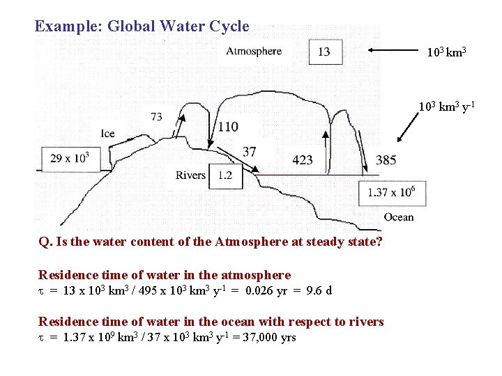
Example: Global Water Cycle 103 km 3 y-1 Q. Is the water content of the Atmosphere at steady state? Residence time of water in the atmosphere = 13 x 103 km 3 / 495 x 103 km 3 y-1 = 0. 026 yr = 9. 6 d Residence time of water in the ocean with respect to rivers = 1. 37 x 109 km 3 / 37 x 103 km 3 y-1 = 37, 000 yrs