Lecture 11 Bayesian Networks CPEN 405 Artificial Intelligence
Lecture 11: Bayesian Networks CPEN 405: Artificial Intelligence Instructor: Robert A. Sowah, Ph. D
Today’s Lecture • Definition of Bayesian networks – Representing a joint distribution by a graph – Can yield an efficient factored representation for a joint distribution • Inference in Bayesian networks – – Inference = answering queries such as P(Q | e) Intractable in general (scales exponentially with num variables) But can be tractable for certain classes of Bayesian networks Efficient algorithms leverage the structure of the graph • Other aspects of Bayesian networks – Real-valued variables – Other types of queries – Special cases: naïve Bayes classifiers, hidden Markov models
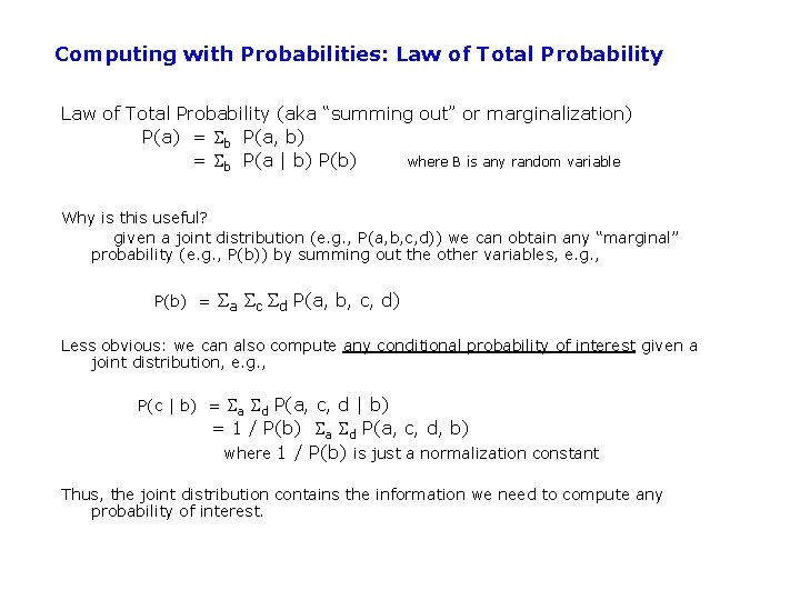
Computing with Probabilities: Law of Total Probability (aka “summing out” or marginalization) P(a) = Sb P(a, b) = Sb P(a | b) P(b) where B is any random variable Why is this useful? given a joint distribution (e. g. , P(a, b, c, d)) we can obtain any “marginal” probability (e. g. , P(b)) by summing out the other variables, e. g. , P(b) = Sa Sc Sd P(a, b, c, d) Less obvious: we can also compute any conditional probability of interest given a joint distribution, e. g. , P(c | b) = Sa Sd P(a, c, d | b) = 1 / P(b) Sa Sd P(a, c, d, b) where 1 / P(b) is just a normalization constant Thus, the joint distribution contains the information we need to compute any probability of interest.

Computing with Probabilities: The Chain Rule or Factoring We can always write P(a, b, c, … z) = P(a | b, c, …. z) P(b, c, … z) (by definition of joint probability) Repeatedly applying this idea, we can write P(a, b, c, … z) = P(a | b, c, …. z) P(b | c, . . z) P(c|. . z). . P(z) This factorization holds for any ordering of the variables This is the chain rule for probabilities
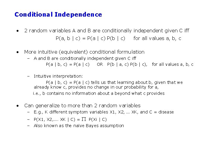
Conditional Independence • 2 random variables A and B are conditionally independent given C iff P(a, b | c) = P(a | c) P(b | c) • for all values a, b, c More intuitive (equivalent) conditional formulation – A and B are conditionally independent given C iff P(a | b, c) = P(a | c) OR P(b | a, c) P(b | c), for all values a, b, c – Intuitive interpretation: P(a | b, c) = P(a | c) tells us that learning about b, given that we already know c, provides no change in our probability for a, i. e. , b contains no information about a beyond what c provides • Can generalize to more than 2 random variables – E. g. , K different symptom variables X 1, X 2, … XK, and C = disease – P(X 1, X 2, …. XK | C) = P(Xi | C) – Also known as the naïve Bayes assumption

“…probability theory is more fundamentally concerned with the structure of reasoning and causation than with numbers. ” Glenn Shafer and Judea Pearl Introduction to Readings in Uncertain Reasoning, Morgan Kaufmann, 1990

Bayesian Networks • A Bayesian network specifies a joint distribution in a structured form • Represent dependence/independence via a directed graph • Structure of the graph Conditional independence relations – Nodes = random variables – Edges = direct dependence In general, p(X 1, X 2, . . XN) = p(Xi | parents(Xi ) ) The full joint distribution The graph-structured approximation • Requires that graph is acyclic (no directed cycles) • 2 components to a Bayesian network – The graph structure (conditional independence assumptions) – The numerical probabilities (for each variable given its parents)
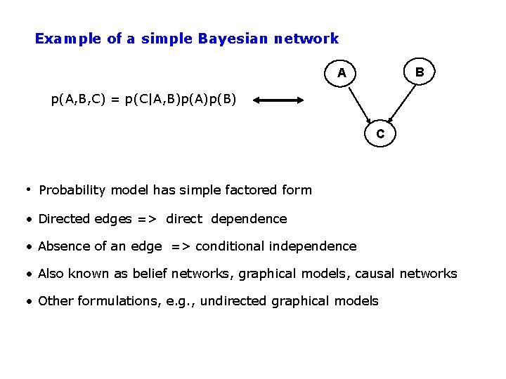
Example of a simple Bayesian network B A p(A, B, C) = p(C|A, B)p(A)p(B) C • Probability model has simple factored form • Directed edges => direct dependence • Absence of an edge => conditional independence • Also known as belief networks, graphical models, causal networks • Other formulations, e. g. , undirected graphical models
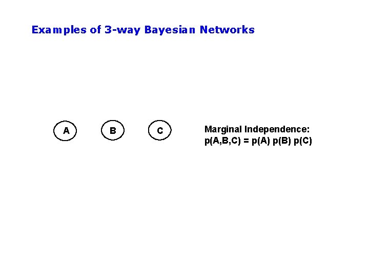
Examples of 3 -way Bayesian Networks A B C Marginal Independence: p(A, B, C) = p(A) p(B) p(C)
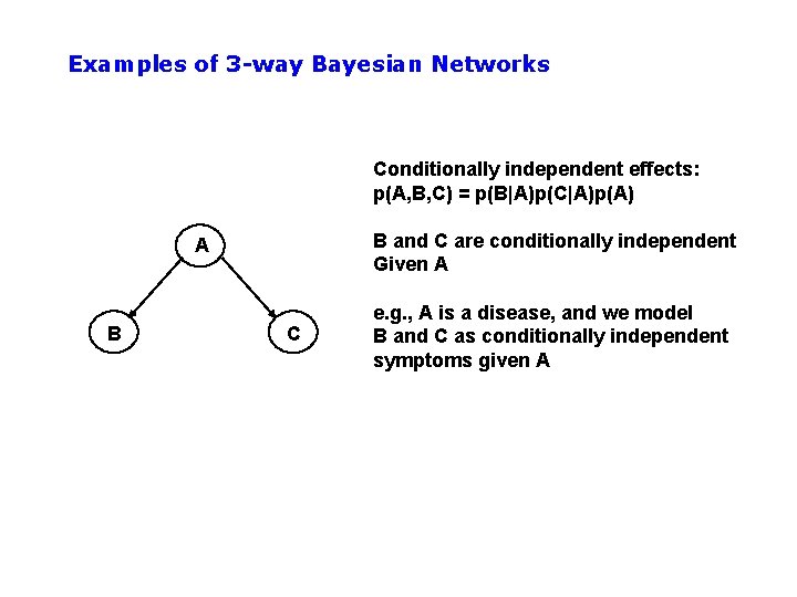
Examples of 3 -way Bayesian Networks Conditionally independent effects: p(A, B, C) = p(B|A)p(C|A)p(A) B and C are conditionally independent Given A A B C e. g. , A is a disease, and we model B and C as conditionally independent symptoms given A
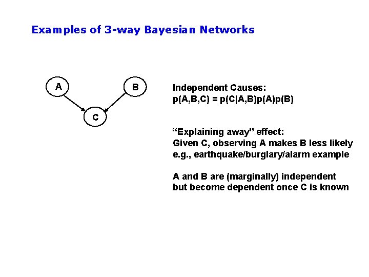
Examples of 3 -way Bayesian Networks A B Independent Causes: p(A, B, C) = p(C|A, B)p(A)p(B) C “Explaining away” effect: Given C, observing A makes B less likely e. g. , earthquake/burglary/alarm example A and B are (marginally) independent but become dependent once C is known
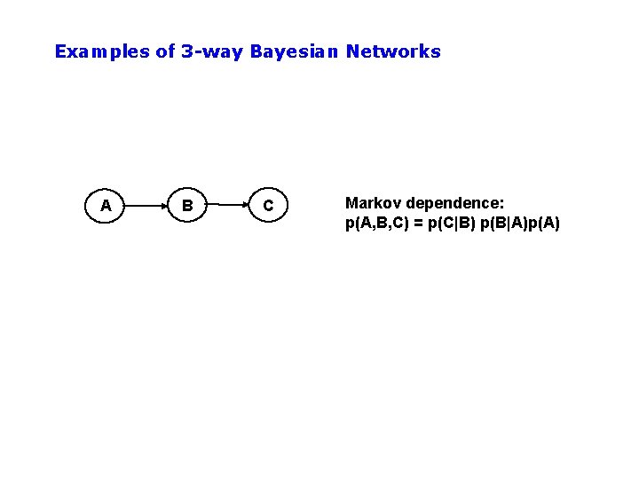
Examples of 3 -way Bayesian Networks A B C Markov dependence: p(A, B, C) = p(C|B) p(B|A)p(A)
Example • Consider the following 5 binary variables: – – – B = a burglary occurs at your house E = an earthquake occurs at your house A = the alarm goes off J = John calls to report the alarm M = Mary calls to report the alarm – What is P(B | M, J) ? (for example) – We can use the full joint distribution to answer this question • Requires 25 = 32 probabilities • Can we use prior domain knowledge to come up with a Bayesian network that requires fewer probabilities?
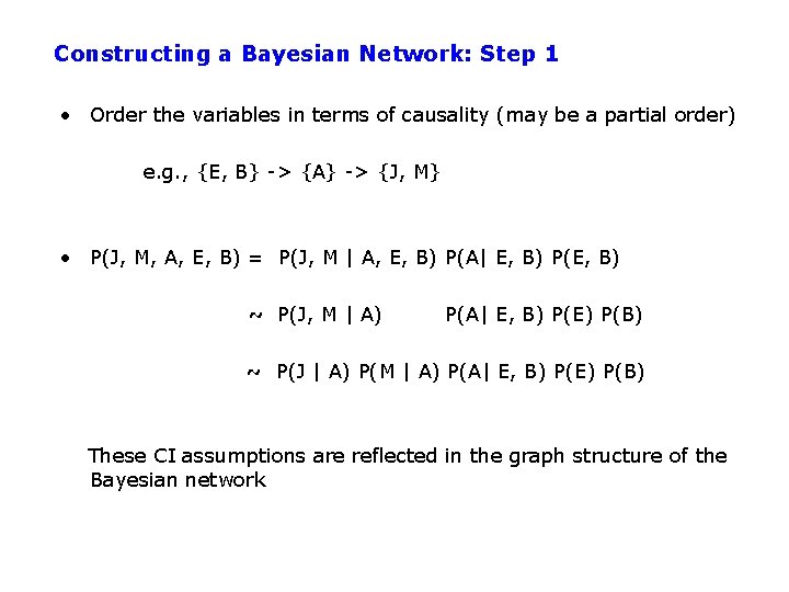
Constructing a Bayesian Network: Step 1 • Order the variables in terms of causality (may be a partial order) e. g. , {E, B} -> {A} -> {J, M} • P(J, M, A, E, B) = P(J, M | A, E, B) P(A| E, B) P(E, B) ~ P(J, M | A) P(A| E, B) P(E) P(B) ~ P(J | A) P(M | A) P(A| E, B) P(E) P(B) These CI assumptions are reflected in the graph structure of the Bayesian network
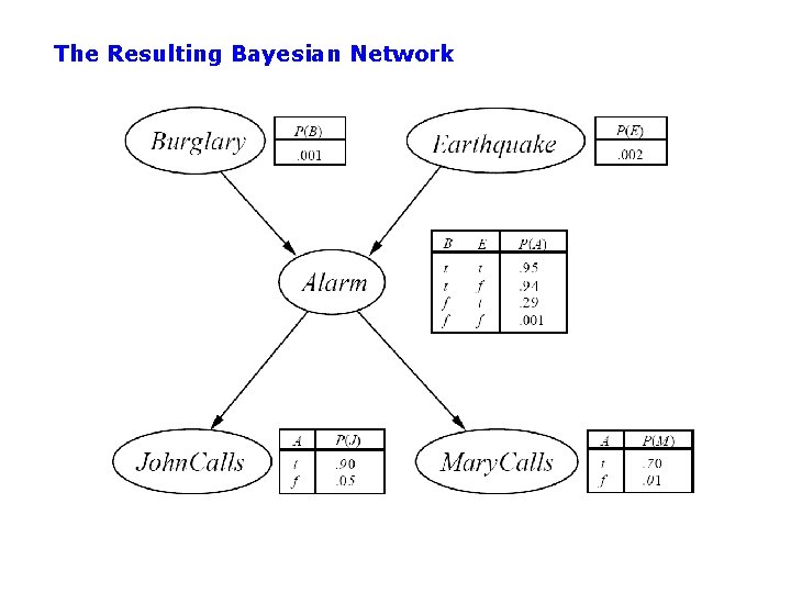
The Resulting Bayesian Network
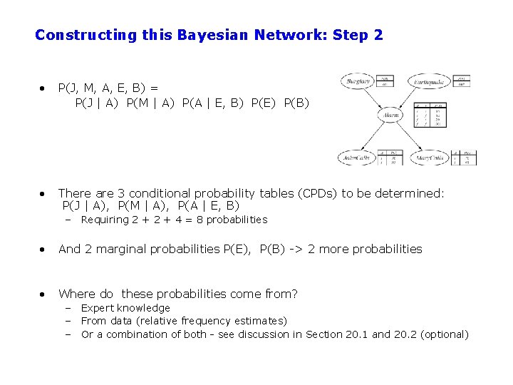
Constructing this Bayesian Network: Step 2 • P(J, M, A, E, B) = P(J | A) P(M | A) P(A | E, B) P(E) P(B) • There are 3 conditional probability tables (CPDs) to be determined: P(J | A), P(M | A), P(A | E, B) – Requiring 2 + 4 = 8 probabilities • And 2 marginal probabilities P(E), P(B) -> 2 more probabilities • Where do these probabilities come from? – Expert knowledge – From data (relative frequency estimates) – Or a combination of both - see discussion in Section 20. 1 and 20. 2 (optional)
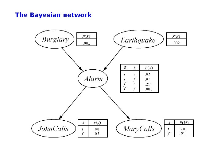
The Bayesian network
Number of Probabilities in Bayesian Networks • Consider n binary variables • Unconstrained joint distribution requires O(2 n) probabilities • If we have a Bayesian network, with a maximum of k parents for any node, then we need O(n 2 k) probabilities • Example – Full unconstrained joint distribution • n = 30: need 109 probabilities for full joint distribution – Bayesian network • n = 30, k = 4: need 480 probabilities
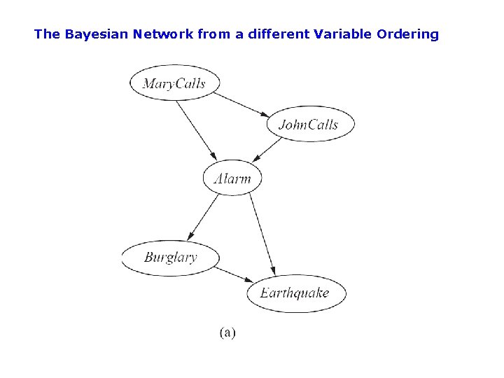
The Bayesian Network from a different Variable Ordering
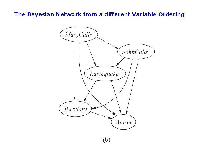
The Bayesian Network from a different Variable Ordering
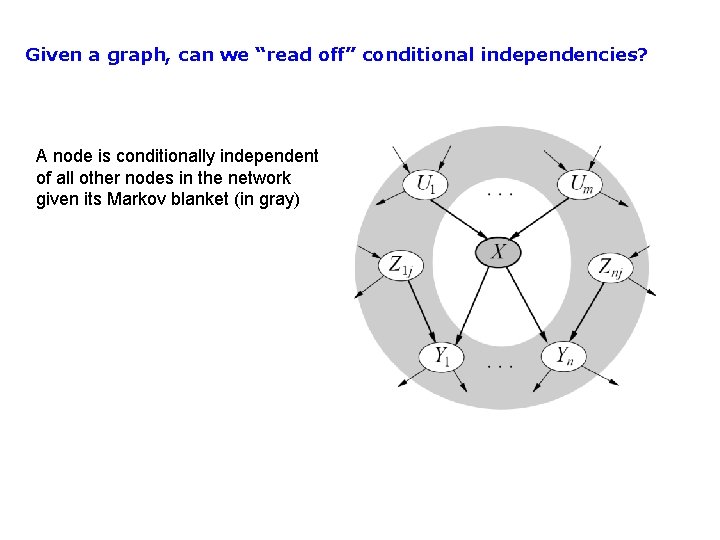
Given a graph, can we “read off” conditional independencies? A node is conditionally independent of all other nodes in the network given its Markov blanket (in gray)
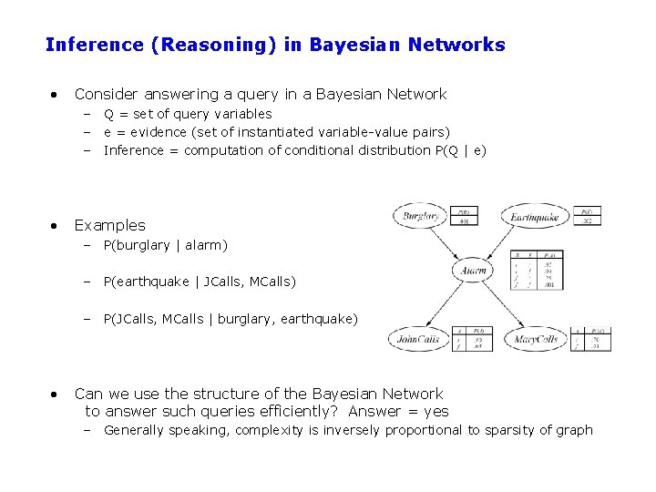
Inference (Reasoning) in Bayesian Networks • Consider answering a query in a Bayesian Network – Q = set of query variables – e = evidence (set of instantiated variable-value pairs) – Inference = computation of conditional distribution P(Q | e) • Examples – P(burglary | alarm) – P(earthquake | JCalls, MCalls) – P(JCalls, MCalls | burglary, earthquake) • Can we use the structure of the Bayesian Network to answer such queries efficiently? Answer = yes – Generally speaking, complexity is inversely proportional to sparsity of graph
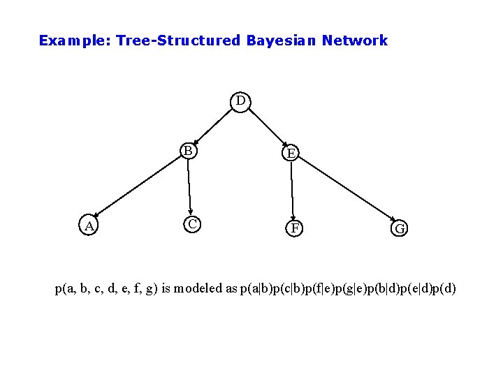
Example: Tree-Structured Bayesian Network D A B E C F G p(a, b, c, d, e, f, g) is modeled as p(a|b)p(c|b)p(f|e)p(g|e)p(b|d)p(e|d)p(d)
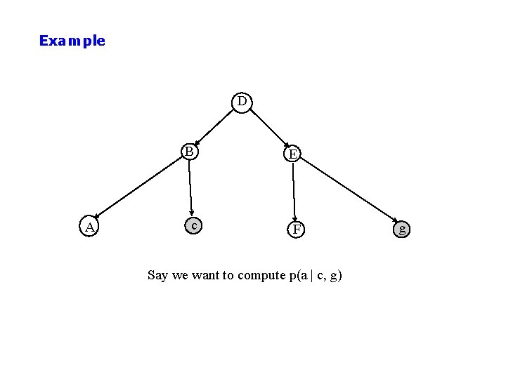
Example D A B E c F Say we want to compute p(a | c, g) g
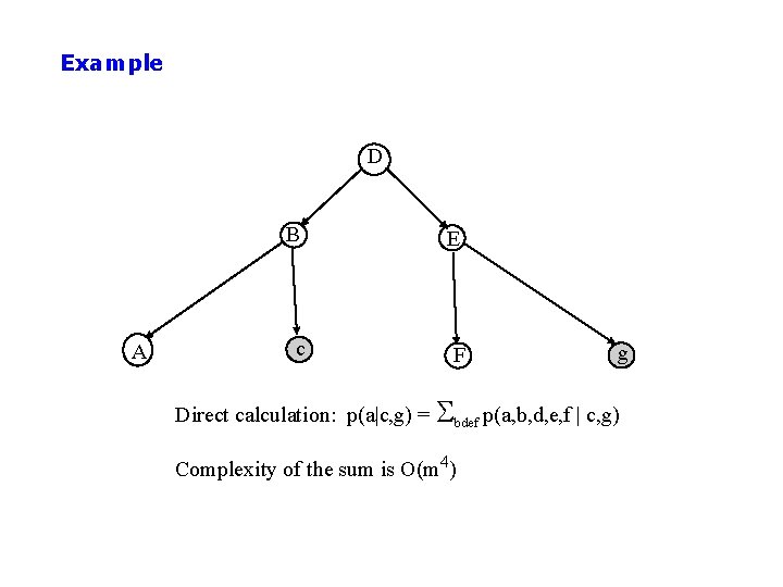
Example D A B E c F g Direct calculation: p(a|c, g) = Sbdef p(a, b, d, e, f | c, g) Complexity of the sum is O(m 4)
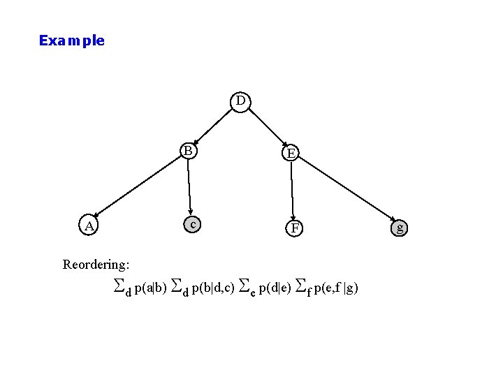
Example D A Reordering: B E c F Sd p(a|b) Sd p(b|d, c) Se p(d|e) Sf p(e, f |g) g
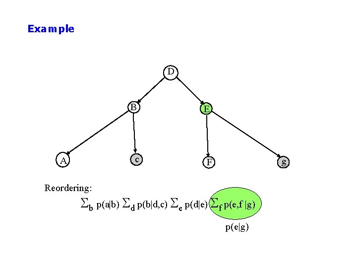
Example D A B E c F g Reordering: Sb p(a|b) Sd p(b|d, c) Se p(d|e) Sf p(e, f |g) p(e|g)

Example D A B E c F Reordering: Sb p(a|b) Sd p(b|d, c) Se p(d|e) p(e|g) p(d|g) g
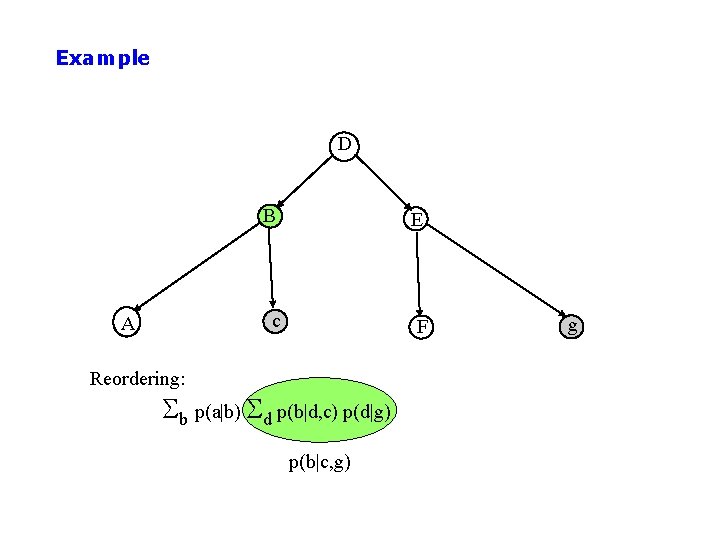
Example D A B E c F Reordering: Sb p(a|b) Sd p(b|d, c) p(d|g) p(b|c, g) g

Example D B E c F A g Reordering: Sb p(a|b) p(b|c, g) p(a|c, g) Complexity is O(m), compared to O(m 4)
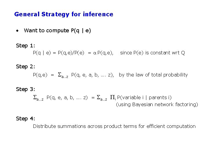
General Strategy for inference • Want to compute P(q | e) Step 1: P(q | e) = P(q, e)/P(e) = a P(q, e), since P(e) is constant wrt Q Step 2: P(q, e) = Sa. . z P(q, e, a, b, …. z), by the law of total probability Step 3: Sa. . z P(q, e, a, b, …. z) = Sa. . z i P(variable i | parents i) (using Bayesian network factoring) Step 4: Distribute summations across product terms for efficient computation

Inference Examples • Examples worked on whiteboard
Complexity of Bayesian Network inference • Assume the network is a polytree – Only a single directed path between any 2 nodes • Complexity scales as O(n m K+1) • n = number of variables • m = arity of variables • K = maximum number of parents for any node – Compare to O(mn-1) for brute-force method • Network is not a polytree? – Can cluster variables to render the new graph a tree – Very similar to tree methods used for – Complexity is O(n m W+1), where W = num variables in largest cluster
Real-valued Variables • Can Bayesian Networks handle Real-valued variables? – If we can assume variables are Gaussian, then the inference and theory for Bayesian networks is well-developed, • E. g. , conditionals of a joint Gaussian is still Gaussian, etc • In inference we replace sums with integrals – For other density functions it depends… • Can often include a univariate variable at the “edge” of a graph, e. g. , a Poisson conditioned on day of week – But for many variables there is little know beyond their univariate properties, e. g. , what would be the joint distribution of a Poisson and a Gaussian? (its not defined) – Common approaches in practice • Put real-valued variables at “leaf nodes” (so nothing is conditioned on them) • Assume real-valued variables are Gaussian or discrete • Discretize real-valued variables
Other aspects of Bayesian Network Inference • The problem of finding an optimal (for inference) ordering and/or clustering of variables for an arbitrary graph is NP-hard – Various heuristics are used in practice – Efficient algorithms and software now exist for working with large Bayesian networks • E. g. , work in Professor Rina Dechter’s group • Other types of queries? – E. g. , finding the most likely values of a variable given evidence – arg max P(Q | e) = “most probable explanation” or maximum a posteriori query - Can also leverage the graph structure in the same manner as for inference – essentially replaces “sum” operator with “max”
Naïve Bayes Model Y 1 Y 2 Y 3 Yn C P(C | Y 1, …Yn) = a P(Yi | C) P (C) Features Y are conditionally independent given the class variable C Widely used in machine learning e. g. , spam email classification: Y’s = counts of words in emails Conditional probabilities P(Yi | C) can easily be estimated from labeled data

Hidden Markov Model (HMM) Y 1 Y 2 Y 3 Yn Observed --------------------------S 1 S 2 S 3 Sn Hidden Two key assumptions: 1. hidden state sequence is Markov 2. observation Yt is CI of all other variables given St Widely used in speech recognition, protein sequence models Since this is a Bayesian network polytree, inference is linear in n
Summary • Bayesian networks represent a joint distribution using a graph • The graph encodes a set of conditional independence assumptions • Answering queries (or inference or reasoning) in a Bayesian network amounts to efficient computation of appropriate conditional probabilities • Probabilistic inference is intractable in the general case – But can be carried out in linear time for certain classes of Bayesian networks

Backup Slides (can be ignored)

Junction Tree D B, E A C F G Good news: can perform MP algorithm on this tree Bad news: complexity is now O(K 2)
A More General Algorithm • Message Passing (MP) Algorithm – Pearl, 1988; Lauritzen and Spiegelhalter, 1988 – Declare 1 node (any node) to be a root – Schedule two phases of message-passing • nodes pass messages up to the root • messages are distributed back to the leaves – In time O(N), we can compute P(…. )
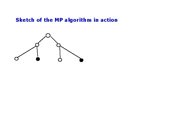
Sketch of the MP algorithm in action

Sketch of the MP algorithm in action 1
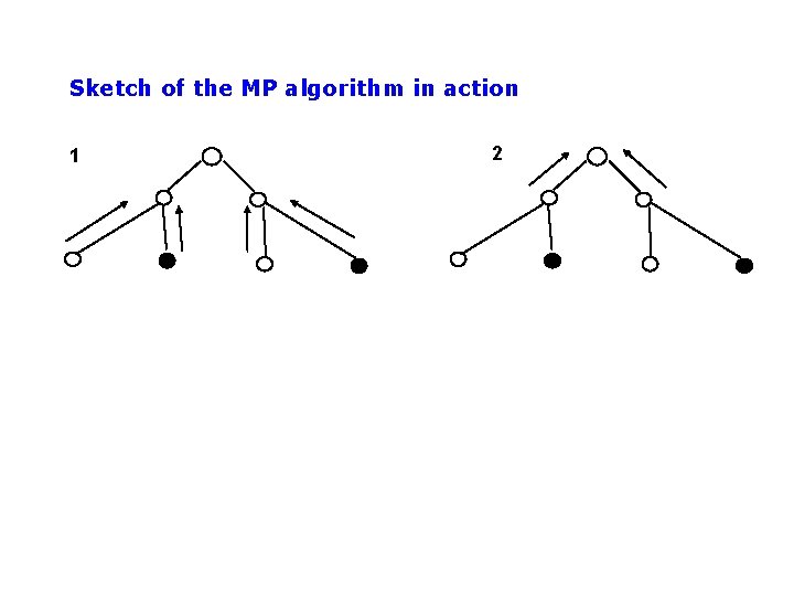
Sketch of the MP algorithm in action 1 2
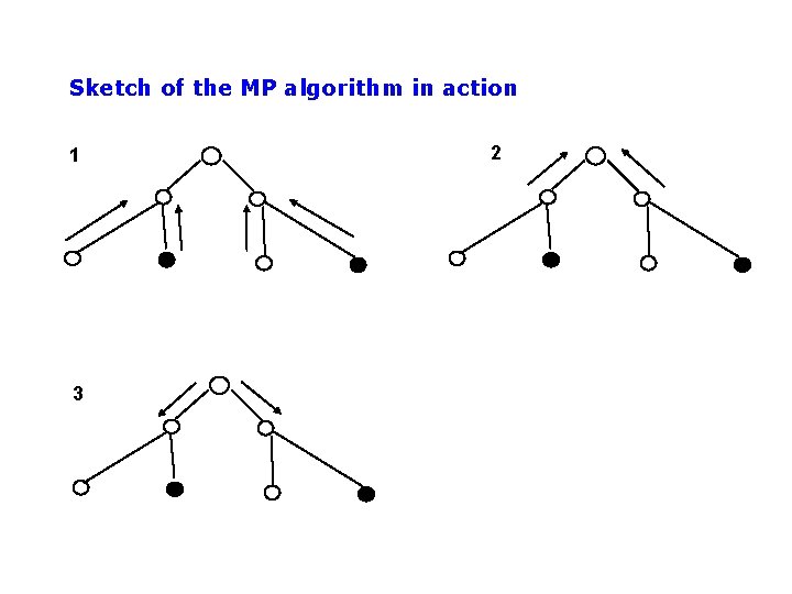
Sketch of the MP algorithm in action 1 3 2
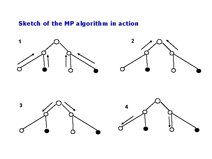
Sketch of the MP algorithm in action 2 1 3 4
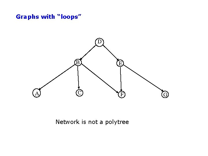
Graphs with “loops” D A B E C F Network is not a polytree G
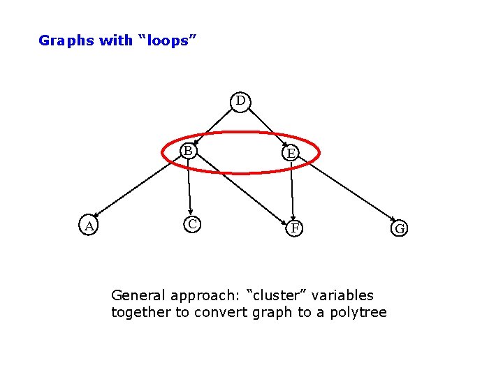
Graphs with “loops” D A B E C F General approach: “cluster” variables together to convert graph to a polytree G
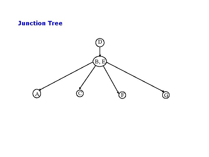
Junction Tree D B, E A C F G
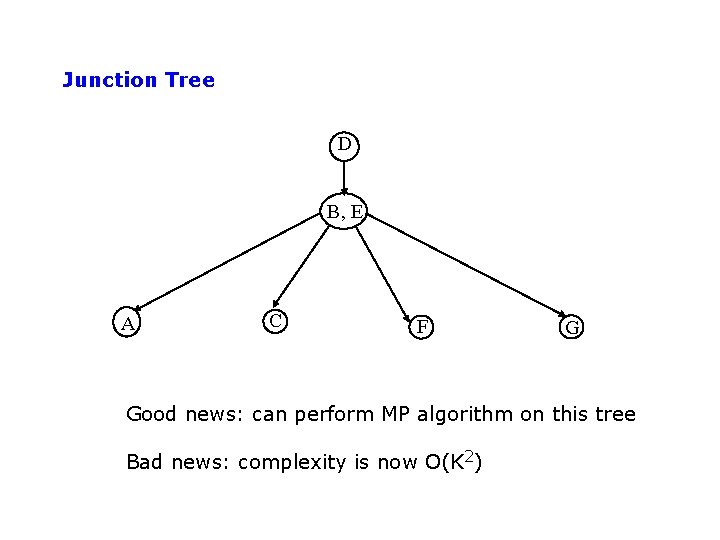
Junction Tree D B, E A C F G Good news: can perform MP algorithm on this tree Bad news: complexity is now O(K 2)
- Slides: 50