Lecture 11 B Trees An IOAware Index Structure

Lecture 11: B+ Trees: An IO-Aware Index Structure

Lecture 11 “If you don’t find it in the index, look very carefully through the entire catalog” - Sears, Roebuck and Co. , Consumers Guide, 1897 2

Lecture 11 Today’s Lecture 1. Indexes: Motivations & Basics 2. B+ Trees 3

Lecture 11 1. Indexes: Motivations & Basics

Lecture 11 > Section 1 What you will learn about in this section 1. Indexes: Motivation 2. Indexes: Basics 3. ACTIVITY: Creating indexes 5

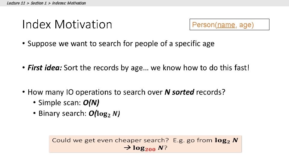
Lecture 11 > Section 1 > Indexes: Motivation Index Motivation • Person(name, age)

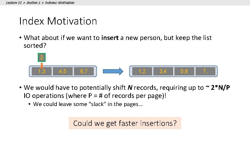
Lecture 11 > Section 1 > Indexes: Motivation Index Motivation • What about if we want to insert a new person, but keep the list sorted? 2 1, 3 4, 5 6, 7 1, 2 3, 4 5, 6 7, • We would have to potentially shift N records, requiring up to ~ 2*N/P IO operations (where P = # of records per page)! • We could leave some “slack” in the pages… Could we get faster insertions?

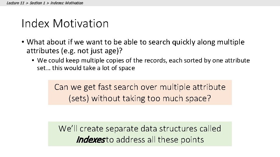
Lecture 11 > Section 1 > Indexes: Motivation Index Motivation • What about if we want to be able to search quickly along multiple attributes (e. g. not just age)? • We could keep multiple copies of the records, each sorted by one attribute set… this would take a lot of space Can we get fast search over multiple attribute (sets) without taking too much space? We’ll create separate data structures called indexes to address all these points

Lecture 11 > Section 1 > Indexes: Motivation Further Motivation for Indexes: No. SQL! • No. SQL engines are (basically) just indexes! • A lot more is left to the user in No. SQL… one of the primary remaining functions of the DBMS is still to provide index over the data records, for the reasons we just saw! • Sometimes use B+ Trees (covered next), sometimes hash indexes (not covered here) Indexes are critical across all DBMS types

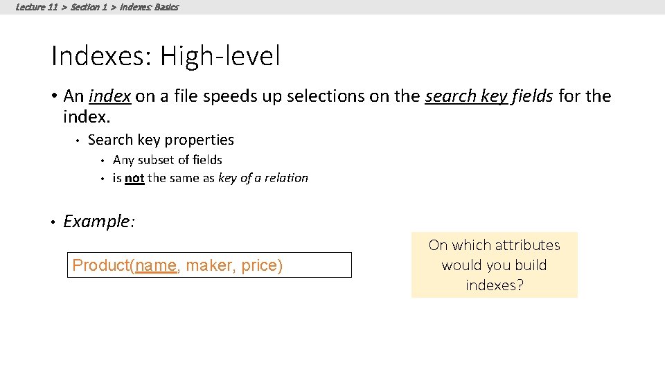
Lecture 11 > Section 1 > Indexes: Basics Indexes: High-level • An index on a file speeds up selections on the search key fields for the index. • Search key properties • • • Any subset of fields is not the same as key of a relation Example: Product(name, maker, price) On which attributes would you build indexes?

Lecture 11 > Section 1 > Indexes: Basics More precisely • An index is a data structure mapping search keys to sets of rows in a database table • • Provides efficient lookup & retrieval by search key value- usually much faster than searching through all the rows of the database table An index can store the full rows it points to (primary index) or pointers to those rows (secondary index) • We’ll mainly consider secondary indexes

Lecture 11 > Section 1 > Indexes: Basics Operations on an Index • Search: Quickly find all records which meet some condition on the search key attributes • More sophisticated variants as well. Why? • Insert / Remove entries • Bulk Load / Delete. Why? Indexing is one the most important features provided by a database for performance

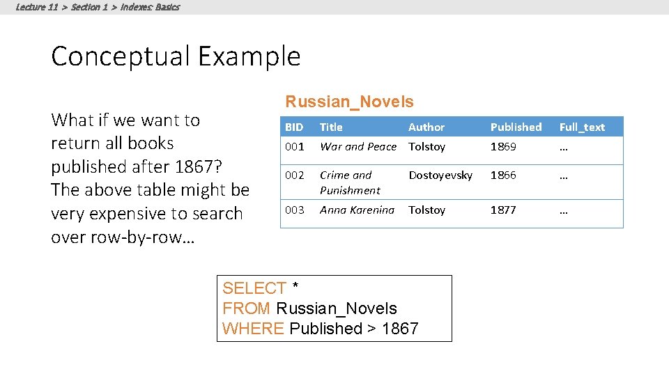
Lecture 11 > Section 1 > Indexes: Basics Conceptual Example What if we want to return all books published after 1867? The above table might be very expensive to search over row-by-row… Russian_Novels BID Title 001 Author Published Full_text War and Peace Tolstoy 1869 … 002 Crime and Punishment Dostoyevsky 1866 … 003 Anna Karenina Tolstoy 1877 … SELECT * FROM Russian_Novels WHERE Published > 1867

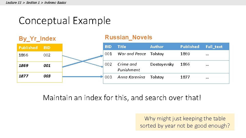
Lecture 11 > Section 1 > Indexes: Basics Conceptual Example By_Yr_Index Russian_Novels Published BID Title 1866 002 001 1869 001 1877 003 Author Published Full_text War and Peace Tolstoy 1869 … 002 Crime and Punishment Dostoyevsky 1866 … 003 Anna Karenina Tolstoy 1877 … Maintain an index for this, and search over that! Why might just keeping the table sorted by year not be good enough?

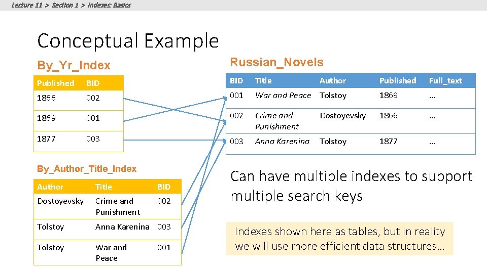
Lecture 11 > Section 1 > Indexes: Basics Conceptual Example By_Yr_Index Russian_Novels Published BID Title 1866 002 001 1869 001 1877 003 By_Author_Title_Index Author Title BID Dostoyevsky Crime and Punishment 002 Tolstoy Anna Karenina 003 Tolstoy War and Peace 001 Author Published Full_text War and Peace Tolstoy 1869 … 002 Crime and Punishment Dostoyevsky 1866 … 003 Anna Karenina Tolstoy 1877 … Can have multiple indexes to support multiple search keys Indexes shown here as tables, but in reality we will use more efficient data structures…

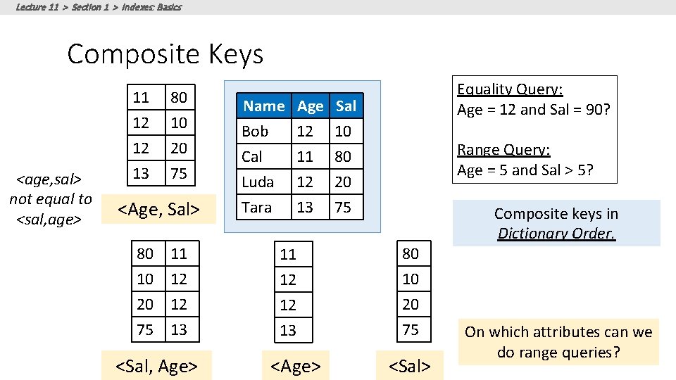
Lecture 11 > Section 1 > Indexes: Basics Composite Keys <age, sal> not equal to <sal, age> 11 12 12 13 80 10 20 75 <Age, Sal> 80 10 20 75 11 12 12 13 <Sal, Age> Name Bob Cal Luda Age 12 11 12 Sal 10 80 20 Tara 13 75 11 12 12 13 <Age> Equality Query: Age = 12 and Sal = 90? Range Query: Age = 5 and Sal > 5? 80 10 20 75 <Sal> Composite keys in Dictionary Order. On which attributes can we do range queries?

Lecture 11 > Section 1 > Indexes: Basics Composite Keys • Pro: • When they work well • We’ll see a good case called “index-only” plans or covering indexes. • Con: • Guesses? (time and space)

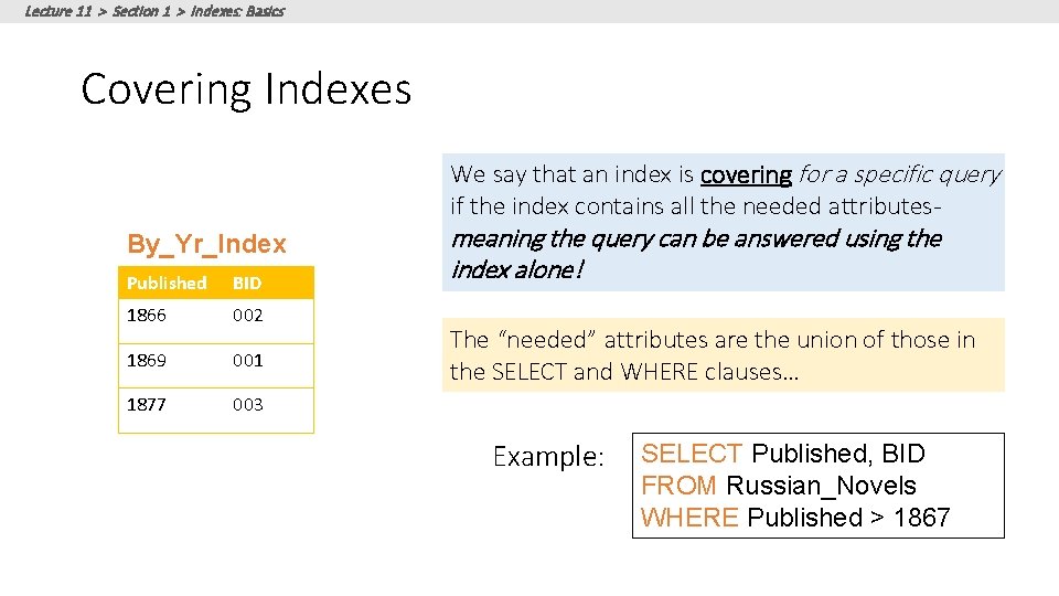
Lecture 11 > Section 1 > Indexes: Basics Covering Indexes We say that an index is covering for a specific query if the index contains all the needed attributes. By_Yr_Index Published BID 1866 002 1869 001 1877 003 meaning the query can be answered using the index alone! The “needed” attributes are the union of those in the SELECT and WHERE clauses… Example: SELECT Published, BID FROM Russian_Novels WHERE Published > 1867

Lecture 11 > Section 1 > Indexes: Basics High-level Categories of Index Types • B-Trees (covered next) • Very good for range queries, sorted data • Some old databases only implemented B-Trees • We will look at a variant called B+ Trees The data structures we present here are “IO aware” • Hash Tables (not covered) • There are variants of this basic structure to deal with IO • Called linear or extendible hashing- IO aware! Real difference between structures: costs of ops determines which index you pick and why

Lecture 11 > Section 1 > ACTIVITY DB-WS 11 a. ipynb 20

Lecture 11 > Section 2 2. B+ Trees 21

Lecture 11 > Section 2 What you will learn about in this section 1. B+ Trees: Basics 2. B+ Trees: Design & Cost 3. Clustered Indexes 22

Lecture 11 > Section 2 > B+ Tree basics B+ Trees • Search trees • B does not mean binary! • Idea in B Trees: • make 1 node = 1 physical page • Balanced, height adjusted tree (not the B either) • Idea in B+ Trees: • Make leaves into a linked list (for range queries)

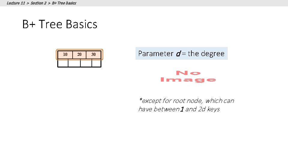
Lecture 11 > Section 2 > B+ Tree basics B+ Tree Basics 10 20 30 Parameter d = the degree *except for root node, which can have between 1 and 2 d keys

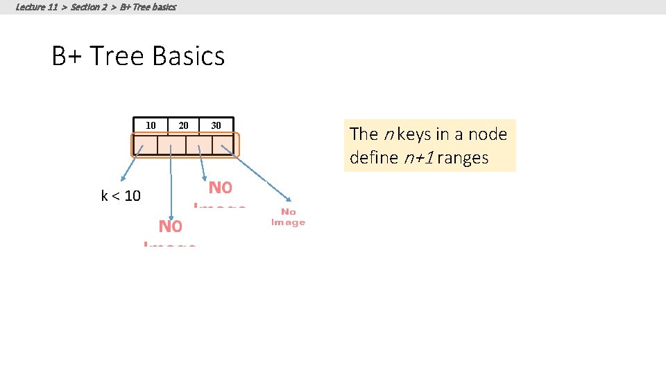
Lecture 11 > Section 2 > B+ Tree basics B+ Tree Basics 10 k < 10 20 30 The n keys in a node define n+1 ranges

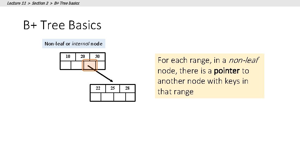
Lecture 11 > Section 2 > B+ Tree basics B+ Tree Basics Non-leaf or internal node 10 20 30 22 25 28 For each range, in a non-leaf node, there is a pointer to another node with keys in that range

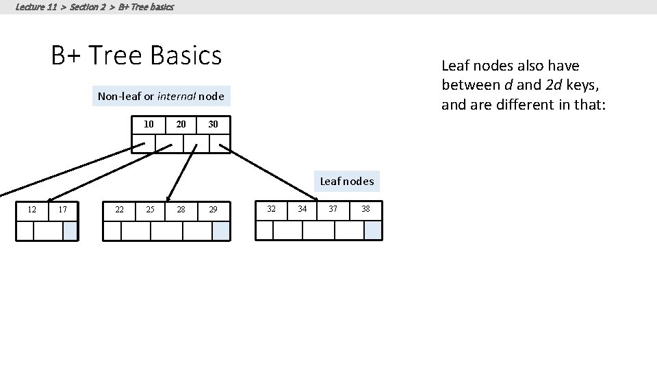
Lecture 11 > Section 2 > B+ Tree basics B+ Tree Basics Leaf nodes also have between d and 2 d keys, and are different in that: Non-leaf or internal node 10 20 30 Leaf nodes 12 17 22 25 28 29 32 34 37 38

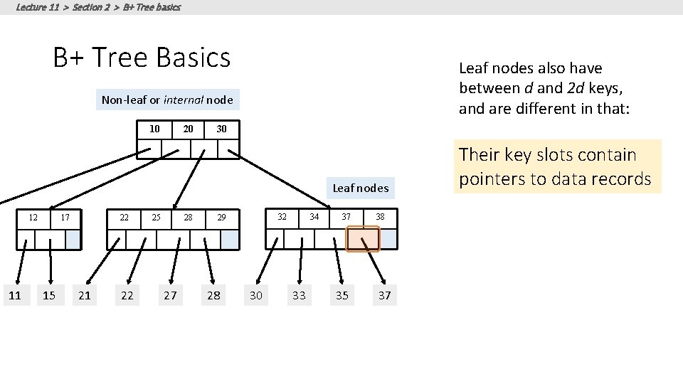
Lecture 11 > Section 2 > B+ Tree basics B+ Tree Basics Leaf nodes also have between d and 2 d keys, and are different in that: Non-leaf or internal node 10 20 30 Leaf nodes 12 11 17 15 22 21 22 25 28 27 32 29 28 30 34 33 37 35 38 37 Their key slots contain pointers to data records

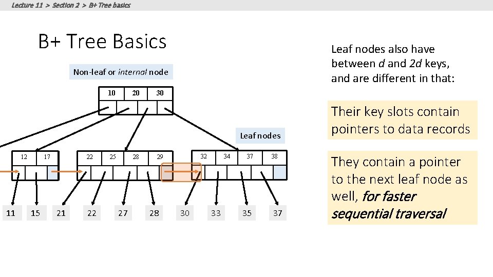
Lecture 11 > Section 2 > B+ Tree basics B+ Tree Basics Leaf nodes also have between d and 2 d keys, and are different in that: Non-leaf or internal node 10 20 30 Leaf nodes 12 11 17 15 22 21 22 25 28 27 32 29 28 30 34 33 37 35 38 37 Their key slots contain pointers to data records They contain a pointer to the next leaf node as well, for faster sequential traversal

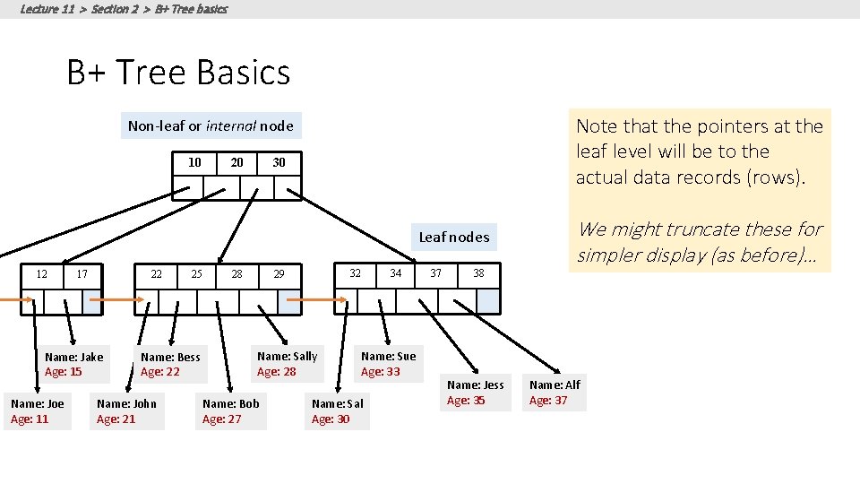
Lecture 11 > Section 2 > B+ Tree basics B+ Tree Basics Note that the pointers at the leaf level will be to the actual data records (rows). Non-leaf or internal node 10 20 30 Leaf nodes 12 17 22 Name: Jake Age: 15 Name: Joe Age: 11 25 Name: Bess Age: 22 Name: John Age: 21 28 32 29 Name: Sally Age: 28 Name: Bob Age: 27 34 Name: Sue Age: 33 Name: Sal Age: 30 37 38 Name: Jess Age: 35 We might truncate these for simpler display (as before)… Name: Alf Age: 37

Lecture 11 > Section 2 > B+ Tree basics Some finer points of B+ Trees

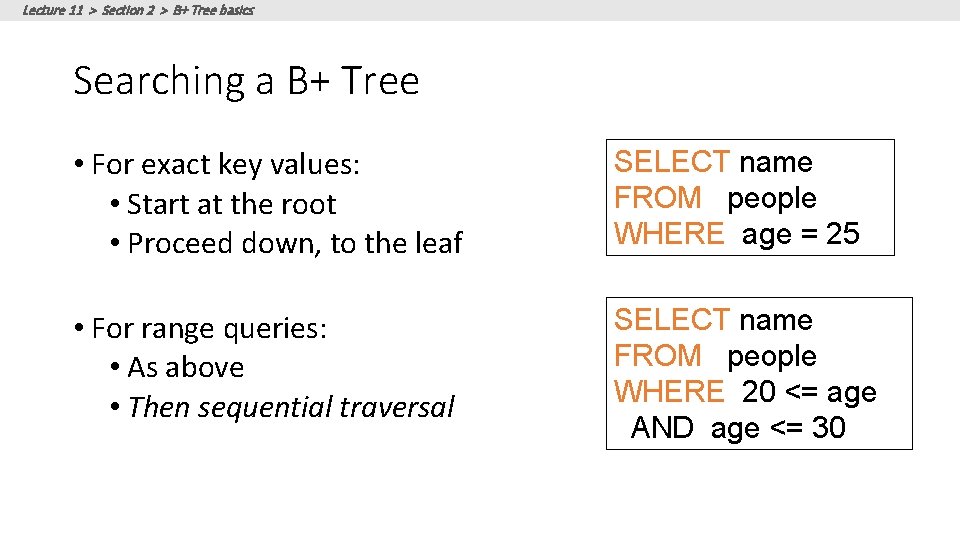
Lecture 11 > Section 2 > B+ Tree basics Searching a B+ Tree • For exact key values: • Start at the root • Proceed down, to the leaf SELECT name FROM people WHERE age = 25 • For range queries: • As above • Then sequential traversal SELECT name FROM people WHERE 20 <= age AND age <= 30

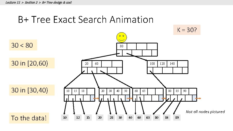
Lecture 11 > Section 2 > B+ Tree design & cost B+ Tree Exact Search Animation 30 < 80 80 30 in [20, 60) 20 30 in [30, 40) To the data! K = 30? 10 15 60 18 100 20 30 40 50 60 120 140 65 80 85 90 Not all nodes pictured 10 12 15 20 28 30 40 60 63 80 84 89

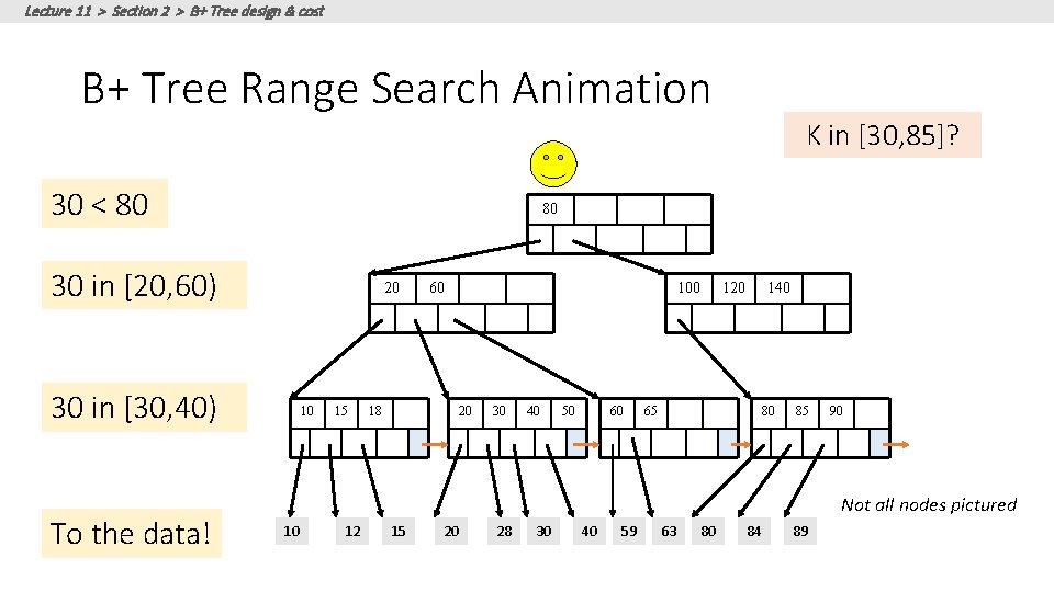
Lecture 11 > Section 2 > B+ Tree design & cost B+ Tree Range Search Animation 30 < 80 80 30 in [20, 60) 20 30 in [30, 40) To the data! K in [30, 85]? 10 15 60 18 100 20 30 40 50 60 120 140 65 80 85 90 Not all nodes pictured 10 12 15 20 28 30 40 59 63 80 84 89

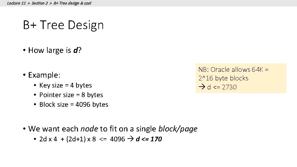
Lecture 11 > Section 2 > B+ Tree design & cost B+ Tree Design • How large is d? • Example: • Key size = 4 bytes • Pointer size = 8 bytes • Block size = 4096 bytes • We want each node to fit on a single block/page • 2 d x 4 + (2 d+1) x 8 <= 4096 d <= 170 NB: Oracle allows 64 K = 2^16 byte blocks d <= 2730

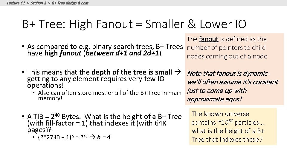
Lecture 11 > Section 2 > B+ Tree design & cost B+ Tree: High Fanout = Smaller & Lower IO The fanout is defined as the • As compared to e. g. binary search trees, B+ Trees number of pointers to child have high fanout (between d+1 and 2 d+1) nodes coming out of a node • This means that the depth of the tree is small Note that fanout is dynamicgetting to any element requires very few IO we’ll often assume it’s constant operations! • Also can often store most or all of the B+ Tree in main just to come up with memory! approximate eqns! • A Ti. B = 240 Bytes. What is the height of a B+ Tree (with fill-factor = 1) that indexes it (with 64 K pages)? • (2*2730 + 1)h = 240 h = 4 The known universe contains ~1080 particles… what is the height of a B+ Tree that indexes these?

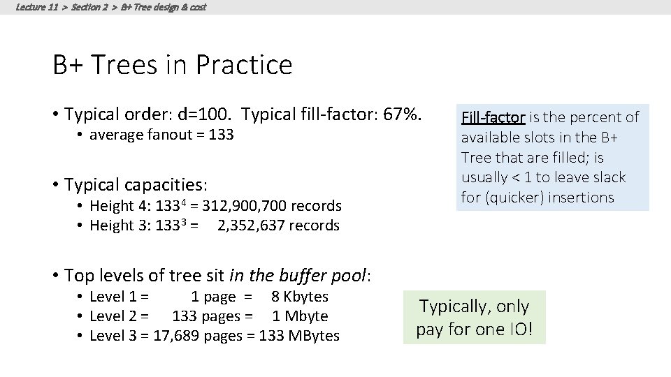
Lecture 11 > Section 2 > B+ Tree design & cost B+ Trees in Practice • Typical order: d=100. Typical fill-factor: 67%. • average fanout = 133 • Typical capacities: • Height 4: 1334 = 312, 900, 700 records • Height 3: 1333 = 2, 352, 637 records Fill-factor is the percent of available slots in the B+ Tree that are filled; is usually < 1 to leave slack for (quicker) insertions • Top levels of tree sit in the buffer pool: • Level 1 = 1 page = 8 Kbytes • Level 2 = 133 pages = 1 Mbyte • Level 3 = 17, 689 pages = 133 MBytes Typically, only pay for one IO!

Lecture 11 > Section 2 > B+ Tree design & cost Simple Cost Model for Search • Let: • f = fanout, which is in [d+1, 2 d+1] (we’ll assume it’s constant for our cost model…) • N = the total number of pages we need to index • F = fill-factor (usually ~= 2/3) • Our B+ Tree needs to have room to index N / F pages! • We have the fill factor in order to leave some open slots for faster insertions • What height (h) does our B+ Tree need to be? • • • h=1 Just the root node- room to index f pages h=2 f leaf nodes- room to index f 2 pages h=3 f 2 leaf nodes- room to index f 3 pages … h fh-1 leaf nodes- room to index fh pages!

Lecture 11 > Section 2 > B+ Tree design & cost Simple Cost Model for Search •

Lecture 11 > Section 2 > B+ Tree design & cost Simple Cost Model for Search • To do range search, we just follow the horizontal pointers • The IO cost is that of loading additional leaf nodes we need to access + the IO cost of loading each page of the results- we phrase this as “Cost(OUT)”

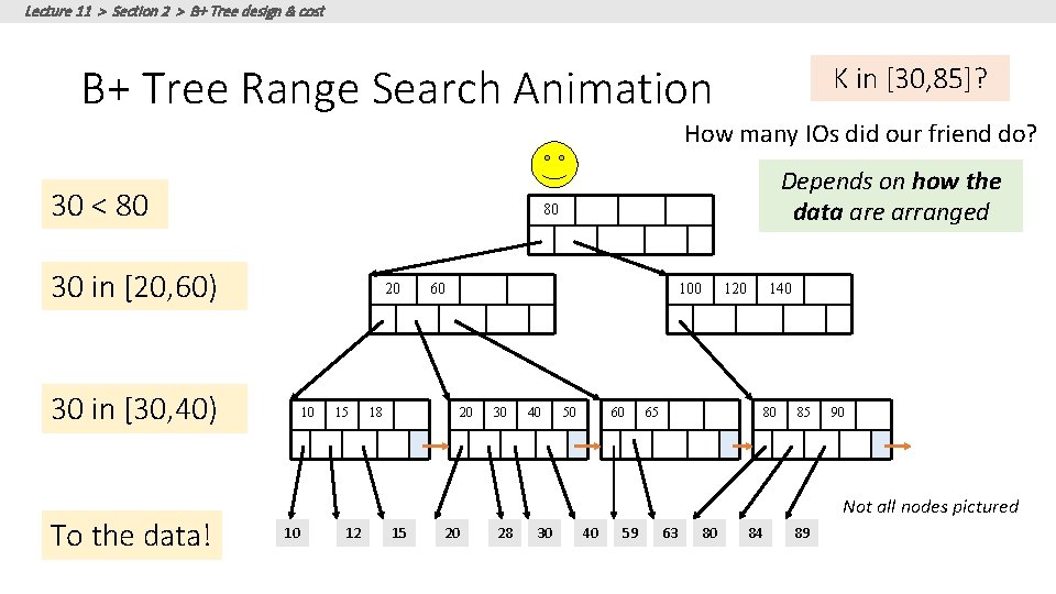
Lecture 11 > Section 2 > B+ Tree design & cost B+ Tree Range Search Animation K in [30, 85]? How many IOs did our friend do? 30 < 80 80 30 in [20, 60) 20 30 in [30, 40) To the data! Depends on how the data are arranged 10 15 60 18 100 20 30 40 50 60 120 140 65 80 85 90 Not all nodes pictured 10 12 15 20 28 30 40 59 63 80 84 89

Lecture 11 > Section 2 > Clustered Indexes An index is clustered if the underlying data is ordered in the same way as the index’s data entries.

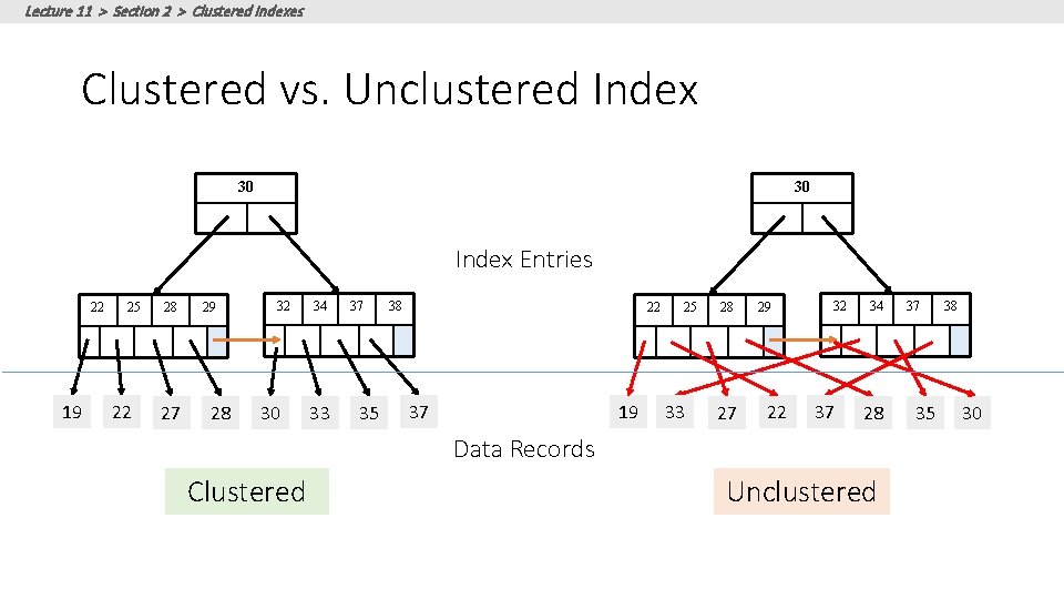
Lecture 11 > Section 2 > Clustered Indexes Clustered vs. Unclustered Index 30 30 Index Entries 22 19 25 22 28 27 29 28 32 30 34 33 37 35 38 22 37 19 25 33 28 27 29 22 32 37 34 28 Data Records Clustered Unclustered 37 35 38 30

Lecture 11 > Section 2 > Clustered Indexes Clustered vs. Unclustered Index • Recall that for a disk with block access, sequential IO is much faster than random IO • For exact search, no difference between clustered / unclustered • For range search over R values: difference between 1 random IO + R sequential IO, and R random IO: • A random IO costs ~ 10 ms (sequential much faster) • For R = 100, 000 records- difference between ~10 ms and ~17 min!

Lecture 11 > Section 2 > B+ Tree design & cost Fast Insertions & Self-Balancing • We won’t go into specifics of B+ Tree insertion algorithm, but has several attractive qualities: • ~ Same cost as exact search • Self-balancing: B+ Tree remains balanced (with respect to height) even after insert B+ Trees also (relatively) fast for single insertions! However, can become bottleneck if many insertions (if fill-factor slack is used up…)

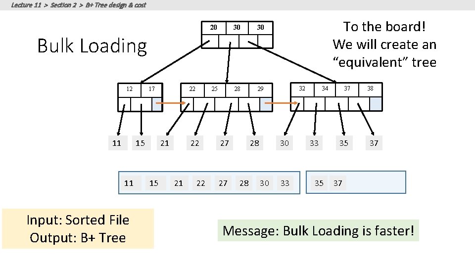
Lecture 11 > Section 2 > B+ Tree design & cost 20 30 30 25 28 29 To the board! We will create an “equivalent” tree Bulk Loading 12 17 15 11 11 Input: Sorted File Output: B+ Tree 22 22 21 15 21 22 27 27 28 28 32 30 30 33 34 33 35 37 35 38 37 37 Message: Bulk Loading is faster!

Lecture 11 > Section 2 > SUMMARY Summary • We covered an algorithm + some optimizations for sorting larger-than -memory files efficiently • An IO aware algorithm! • We create indexes over tables in order to support fast (exact and range) search and insertion over multiple search keys • B+ Trees are one index data structure which support very fast exact and range search & insertion via high fanout • Clustered vs. unclustered makes a big difference for range queries too