Lecture 11 A Divide and Conquer algorithms Implementation

Lecture 11 A Divide and Conquer algorithms Implementation aspects COMP 1100

Acknowledgement of Country ü I wish to acknowledge the traditional custodians of the land we are meeting on, the Ngunnawal people. I wish to acknowledge and respect their continuing culture and the contribution they make to the life of this city and this region. I would also like to acknowledge and welcome any other Aboriginal and Torres Strait Islander people who are enrolled in our courses. 2

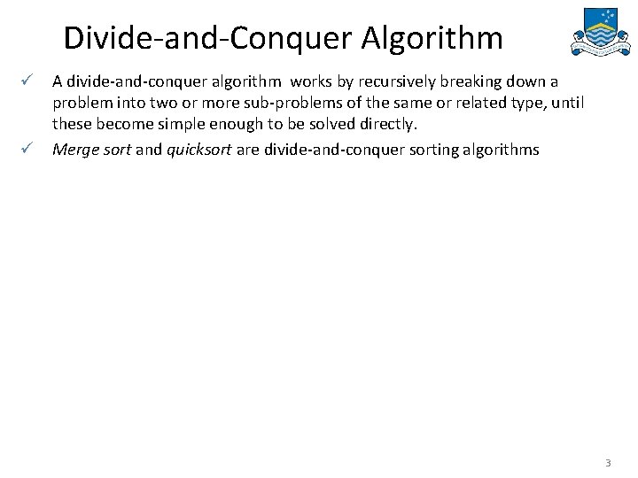
Divide-and-Conquer Algorithm ü A divide-and-conquer algorithm works by recursively breaking down a problem into two or more sub-problems of the same or related type, until these become simple enough to be solved directly. ü Merge sort and quicksort are divide-and-conquer sorting algorithms 3

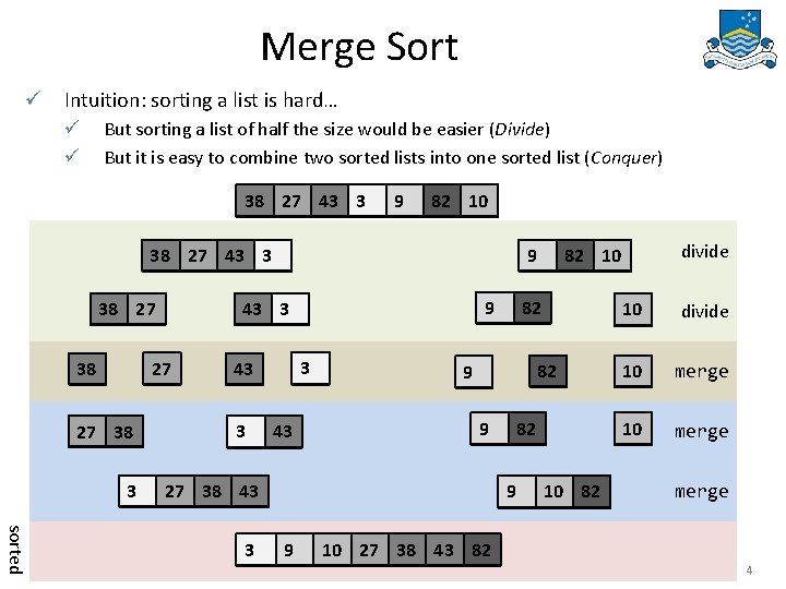
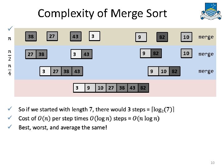
Merge Sort ü Intuition: sorting a list is hard… ü ü But sorting a list of half the size would be easier (Divide) But it is easy to combine two sorted lists into one sorted list (Conquer) 38 27 43 3 9 82 10 38 27 43 3 38 27 27 38 3 9 43 3 27 38 9 3 43 82 9 27 38 43 sorted 3 82 9 9 divide 82 10 10 82 10 divide 10 merge 10 27 38 43 82 4

Merge merge : : Ord a => [a] -> [a] merge list 1 list 2 = case (list 1, list 2) of (list, []) -> list ([], list) -> list (x: xs, y: ys) | x <= y -> x : merge xs (y: ys) | otherwise -> y : merge (x: xs) ys 9 9 82 9 <= 10 9 10 10 82 9 : merge (82: []) (10: []) 1 comparison merge [9, 82] [10] = {applying merge} = {applying (list 1, list 2)} ([9, 82], [10]) = {applying (x: xs, y: ys)} (9: (82: []), 10: []) = {applying x <= y and guard} 9 : merge (82: []) (10: []) = {applying merge} = {applying (list 1, list 2)} ([82], [10]) = {applying (x: xs, y: ys)} ((82: []), (10: [])) = {applying x <= y and guard} 10 : merge (82: []) ([]) = {applying merge} = {applying (list 1, list 2)} ([82], []) = {applying the base case} ((82: []), []) -> (82: []) = {applying cons} 10: (82: []) = {applying cons} 9: (10: (82: [])) 5

Complexity of Merge ü 5 9 14 17 5 9 5 [] 14 17 9 14 17 5 5 5 14 17 9 14 17 [] 9 5 9 9 14 17 6

Complexity of Merge ü 5 14 9 17 5 9 14 [] 17 5 9 14 17 7

Merge Sort merge. Sort : : Ord a => [a] -> [a] merge. Sort list = case list of [] -> [] [x] -> [x] _ -> merge (merge. Sort first. Half) (merge. Sort second. Half) where first. Half = take half list second. Half = drop half list half = div (length list) 2 8

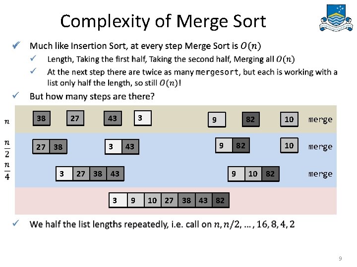
Complexity of Merge Sort ü 27 38 3 3 43 82 9 9 27 38 43 3 82 9 9 10 82 10 merge 10 27 38 43 82 9

Complexity of Merge Sort ü 27 38 3 3 43 82 9 9 27 38 43 3 82 9 9 10 82 10 merge 10 27 38 43 82 10

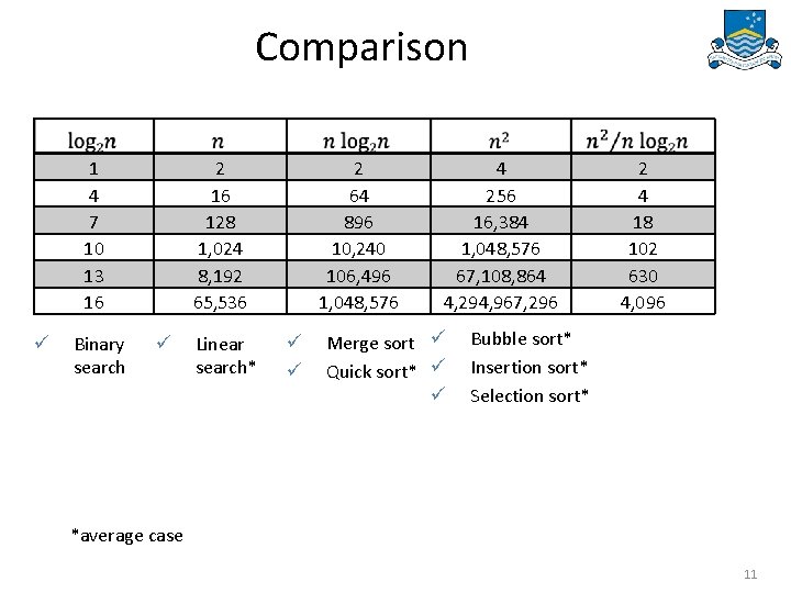
Comparison 1 4 7 10 13 16 ü Binary search 2 16 128 1, 024 8, 192 65, 536 ü Linear search* 2 64 896 10, 240 106, 496 1, 048, 576 ü ü 4 256 16, 384 1, 048, 576 67, 108, 864 4, 294, 967, 296 Merge sort ü Quick sort* ü ü 2 4 18 102 630 4, 096 Bubble sort* Insertion sort* Selection sort* *average case 11

Comparison of Sorting Algorithms ü quick. Sort : : [Integer] -> [Integer] quick. Sort [] = [] quick. Sort (x: xs) = quick. Sort smaller ++ [x] ++ quick. Sort larger where smaller = [a | a <- xs, a <= x] larger = [b | b <- xs, b > x] 12

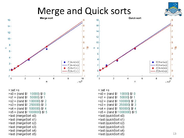
Merge and Quick sorts >: set +s >s 0 = (rand $! 10000) $! 0 >s 1 = (rand $! 50000) $! 1 >s 2 = (rand $! 100000) $! 2 >s 3 = (rand $! 250000) $! 3 >s 4 = (rand $! 500000) $! 4 >s 5 = (rand $! 1000000) $! 5 >last (merge. Sort s 0) >last (merge. Sort s 1) >last (merge. Sort s 2) >last (merge. Sort s 3) >last (merge. Sort s 4) >last (merge. Sort s 5) >: set +s >s 0 = (rand $! 10000) $! 0 >s 1 = (rand $! 50000) $! 1 >s 2 = (rand $! 100000) $! 2 >s 3 = (rand $! 250000) $! 3 >s 4 = (rand $! 500000) $! 4 >s 5 = (rand $! 1000000) $! 5 >last (quick. Sort s 0) >last (quick. Sort s 1) >last (quick. Sort s 2) >last (quick. Sort s 3) >last (quick. Sort s 4) >last (quick. Sort s 5) 13

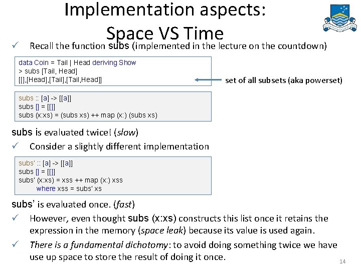
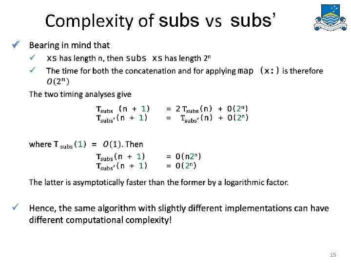
ü Implementation aspects: Space VS Time Recall the function subs (implemented in the lecture on the countdown) data Coin = Tail | Head deriving Show > subs [Tail, Head] [[], [Head], [Tail, Head]] set of all subsets (aka powerset) subs : : [a] -> [[a]] subs [] = [[]] subs (x: xs) = (subs xs) ++ map (x: ) (subs xs) subs is evaluated twice! (slow) ü Consider a slightly different implementation subs’ : : [a] -> [[a]] subs [] = [[]] subs’ (x: xs) = xss ++ map (x: ) xss where xss = subs’ xs subs’ is evaluated once. (fast) ü However, even thought subs (x: xs) constructs this list once it retains the expression in the memory (space leak) because its value is used again. ü There is a fundamental dichotomy: to avoid doing something twice we have use up space to store the result of doing it once. 14

Complexity of subs vs subs’ ü 15

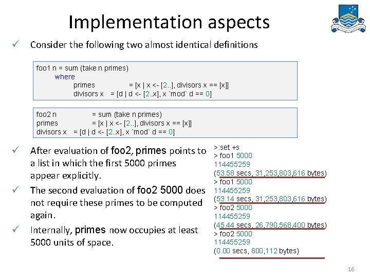
Implementation aspects ü Consider the following two almost identical definitions foo 1 n = sum (take n primes) where primes = [x | x <- [2. . ], divisors x == [x]] divisors x = [d | d <- [2. . x], x `mod` d == 0] foo 2 n = sum (take n primes) primes = [x | x <- [2. . ], divisors x == [x]] divisors x = [d | d <- [2. . x], x `mod` d == 0] ü After evaluation of foo 2, primes points to a list in which the first 5000 primes appear explicitly. ü The second evaluation of foo 2 5000 does not require these primes to be computed again. ü Internally, primes now occupies at least 5000 units of space. >: set +s > foo 1 5000 114455259 (53. 58 secs, 31, 253, 803, 616 bytes) > foo 1 5000 114455259 (53. 14 secs, 31, 253, 803, 616 bytes) > foo 2 5000 114455259 (45. 44 secs, 26, 790, 568, 400 bytes) > foo 2 5000 114455259 (0. 00 secs, 800, 112 bytes) 16

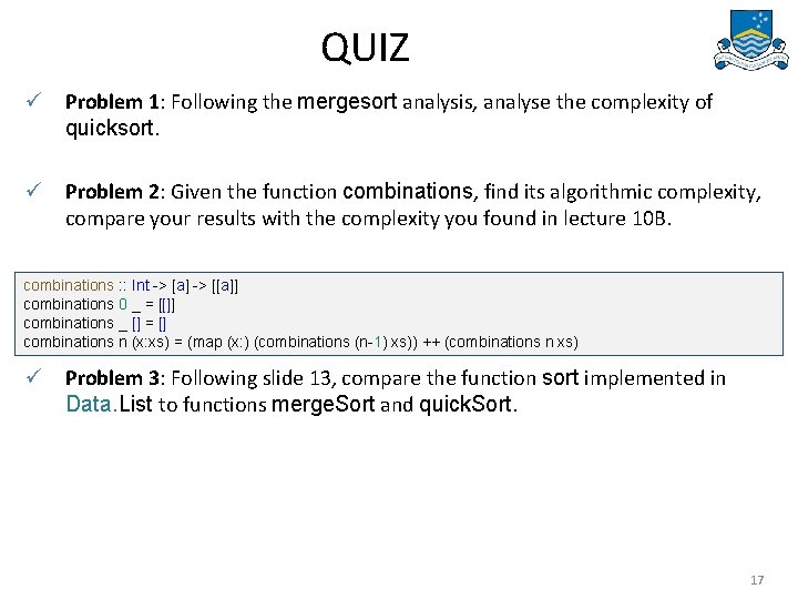
QUIZ ü Problem 1: Following the mergesort analysis, analyse the complexity of quicksort. ü Problem 2: Given the function combinations, find its algorithmic complexity, compare your results with the complexity you found in lecture 10 B. ü ] combinations : : Int -> [a] -> [[a]] combinations 0 _ = [[]] combinations _ [] = [] combinations n (x: xs) = (map (x: ) (combinations (n-1) xs)) ++ (combinations n xs) ü Problem 3: Following slide 13, compare the function sort implemented in Data. List to functions merge. Sort and quick. Sort. 17