Lecture 10 Simulation Techniques How to generate samples

Lecture 10 Simulation Techniques How to generate samples from posterior The future is completely uncertain… …I am completely certain of this

Simulation Techniques • Summary of the methods we used so far • Other methods – Rejection sampling – Importance sampling 2 Structural & Multidisciplinary Optimization Group

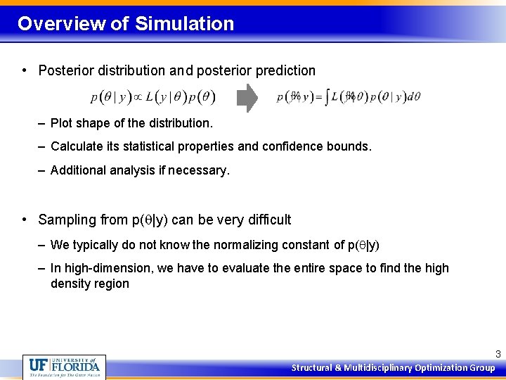
Overview of Simulation • Posterior distribution and posterior prediction – Plot shape of the distribution. – Calculate its statistical properties and confidence bounds. – Additional analysis if necessary. • Sampling from p(q|y) can be very difficult – We typically do not know the normalizing constant of p(q|y) – In high-dimension, we have to evaluate the entire space to find the high density region 3 Structural & Multidisciplinary Optimization Group

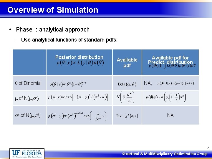
Overview of Simulation • Phase I: analytical approach – Use analytical functions of standard pdfs. Posterior distribution q of Binomial Available pdf for Predict. distribution NA, m of N(m, s 2) s 2 of N(m, s 2) NA 4 Structural & Multidisciplinary Optimization Group

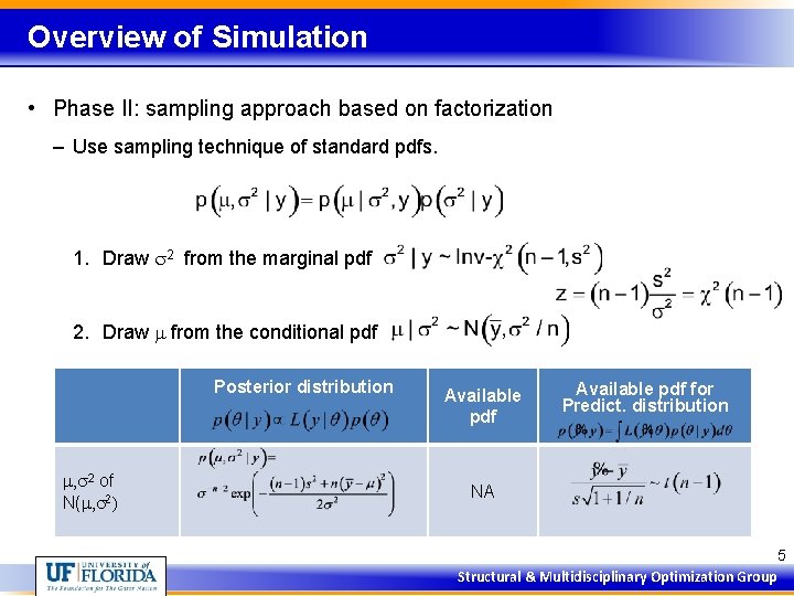
Overview of Simulation • Phase II: sampling approach based on factorization – Use sampling technique of standard pdfs. 1. Draw s 2 from the marginal pdf 2. Draw m from the conditional pdf Posterior distribution m, s 2 of N(m, s 2) Available pdf for Predict. distribution NA 5 Structural & Multidisciplinary Optimization Group

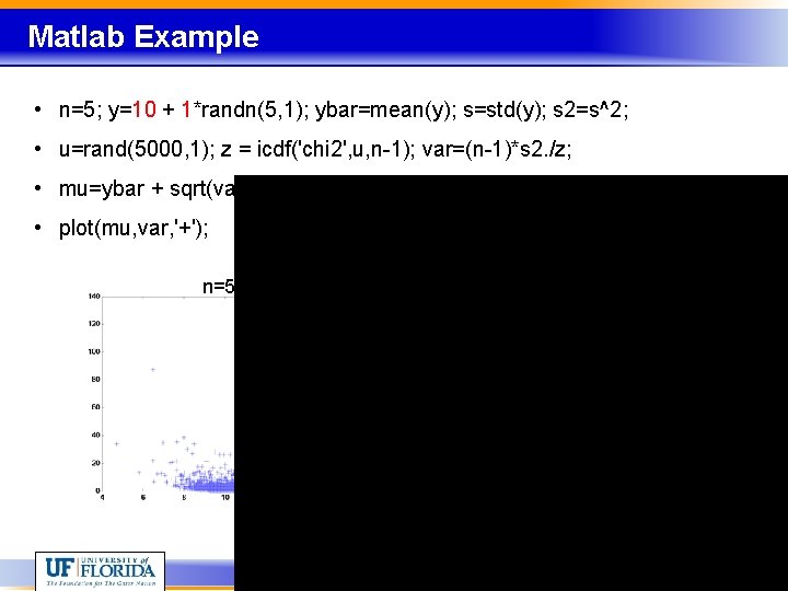
Matlab Example • n=5; y=10 + 1*randn(5, 1); ybar=mean(y); s=std(y); s 2=s^2; • u=rand(5000, 1); z = icdf('chi 2', u, n-1); var=(n-1)*s 2. /z; • mu=ybar + sqrt(var. /n). *randn(NS, 1); • plot(mu, var, '+'); n=5 n=10 6 Structural & Multidisciplinary Optimization Group

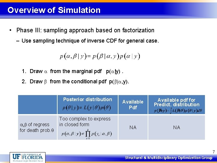
Overview of Simulation • Phase III: sampling approach based on factorization – Use sampling technique of inverse CDF for general case. 1. Draw a from the marginal pdf p(a|y). 2. Draw b from the conditional pdf p(b|a, y). Posterior distribution a, b of regress for death prob. q Too complex to express in closed form Available Pdf Available pdf for Predict. distribution NA NA 7 Structural & Multidisciplinary Optimization Group

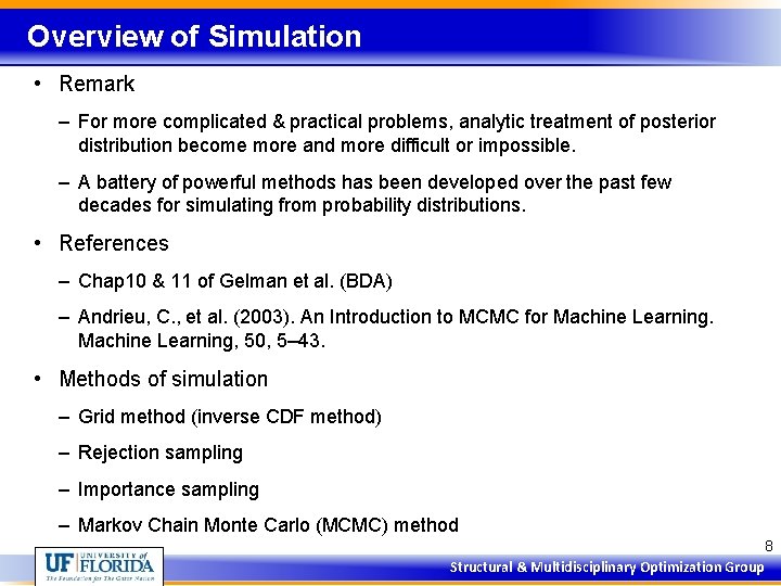
Overview of Simulation • Remark – For more complicated & practical problems, analytic treatment of posterior distribution become more and more difficult or impossible. – A battery of powerful methods has been developed over the past few decades for simulating from probability distributions. • References – Chap 10 & 11 of Gelman et al. (BDA) – Andrieu, C. , et al. (2003). An Introduction to MCMC for Machine Learning, 50, 5– 43. • Methods of simulation – Grid method (inverse CDF method) – Rejection sampling – Importance sampling – Markov Chain Monte Carlo (MCMC) method 8 Structural & Multidisciplinary Optimization Group

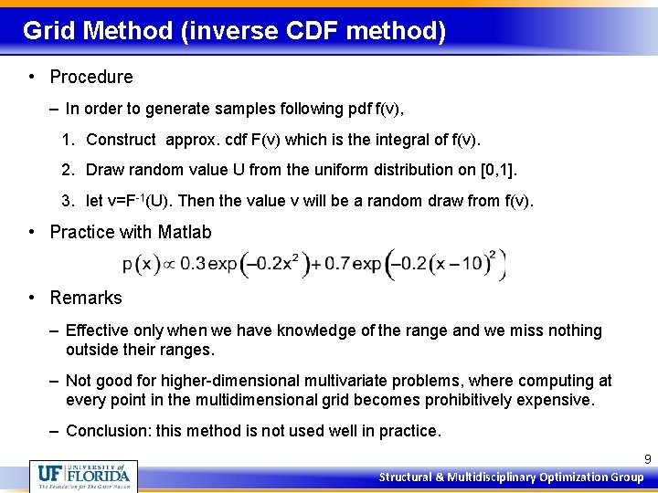
Grid Method (inverse CDF method) • Procedure – In order to generate samples following pdf f(v), 1. Construct approx. cdf F(v) which is the integral of f(v). 2. Draw random value U from the uniform distribution on [0, 1]. 3. let v=F-1(U). Then the value v will be a random draw from f(v). • Practice with Matlab • Remarks – Effective only when we have knowledge of the range and we miss nothing outside their ranges. – Not good for higher-dimensional multivariate problems, where computing at every point in the multidimensional grid becomes prohibitively expensive. – Conclusion: this method is not used well in practice. 9 Structural & Multidisciplinary Optimization Group

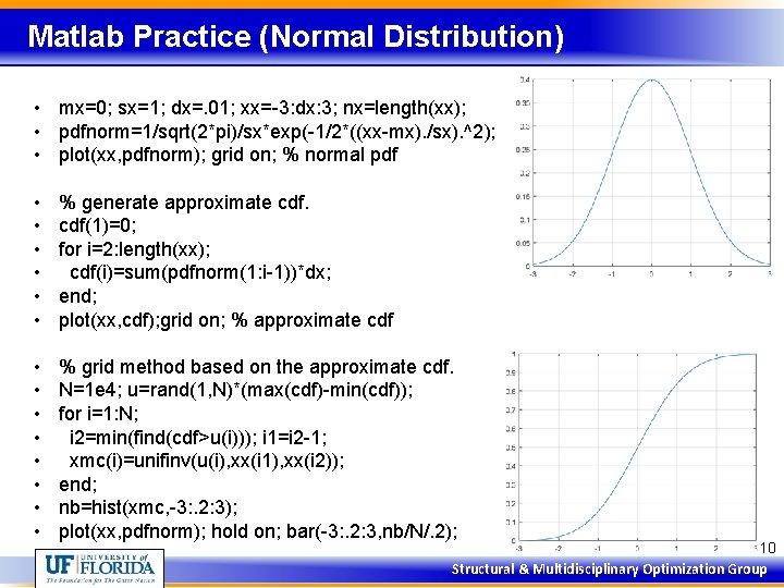
Matlab Practice (Normal Distribution) • mx=0; sx=1; dx=. 01; xx=-3: dx: 3; nx=length(xx); • pdfnorm=1/sqrt(2*pi)/sx*exp(-1/2*((xx-mx). /sx). ^2); • plot(xx, pdfnorm); grid on; % normal pdf • • • % generate approximate cdf(1)=0; for i=2: length(xx); cdf(i)=sum(pdfnorm(1: i-1))*dx; end; plot(xx, cdf); grid on; % approximate cdf • • % grid method based on the approximate cdf. N=1 e 4; u=rand(1, N)*(max(cdf)-min(cdf)); for i=1: N; i 2=min(find(cdf>u(i))); i 1=i 2 -1; xmc(i)=unifinv(u(i), xx(i 1), xx(i 2)); end; nb=hist(xmc, -3: . 2: 3); plot(xx, pdfnorm); hold on; bar(-3: . 2: 3, nb/N/. 2); 10 Structural & Multidisciplinary Optimization Group

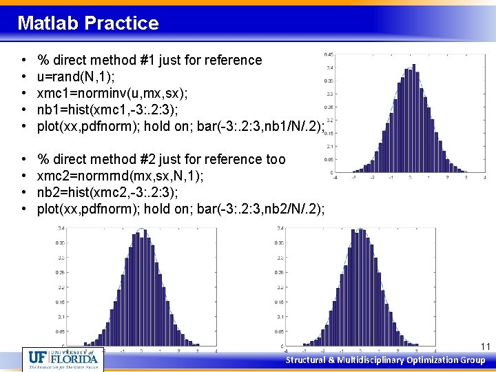
Matlab Practice • • • % direct method #1 just for reference u=rand(N, 1); xmc 1=norminv(u, mx, sx); nb 1=hist(xmc 1, -3: . 2: 3); plot(xx, pdfnorm); hold on; bar(-3: . 2: 3, nb 1/N/. 2); • • % direct method #2 just for reference too xmc 2=normrnd(mx, sx, N, 1); nb 2=hist(xmc 2, -3: . 2: 3); plot(xx, pdfnorm); hold on; bar(-3: . 2: 3, nb 2/N/. 2); 11 Structural & Multidisciplinary Optimization Group

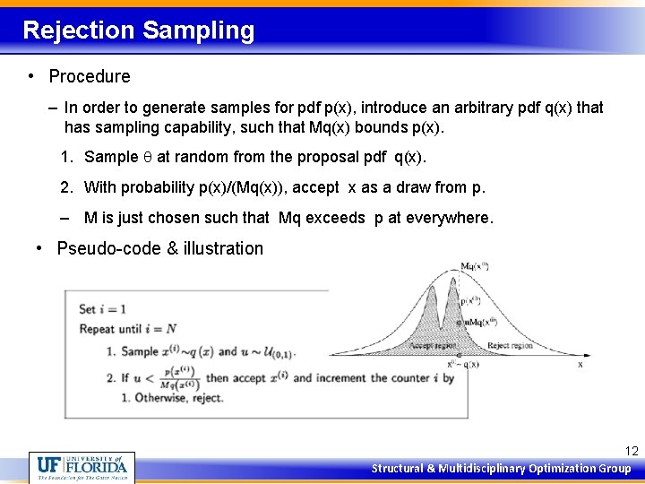
Rejection Sampling • Procedure – In order to generate samples for pdf p(x), introduce an arbitrary pdf q(x) that has sampling capability, such that Mq(x) bounds p(x). 1. Sample q at random from the proposal pdf q(x). 2. With probability p(x)/(Mq(x)), accept x as a draw from p. – M is just chosen such that Mq exceeds p at everywhere. • Pseudo-code & illustration 12 Structural & Multidisciplinary Optimization Group

Triangular Distribution Example Mq(x) • p(x)=2 x for x in [0, 1] – Select q(x)=U[0, 1] p(x) – Then M=3 is large enough. q(x) 0 1 qsamp=rand(1, 5) = 0. 8147 0. 9058 0. 1270 0. 9134 0. 6324. px=2*qsamp = 1. 6294 1. 8116 0. 2540 1. 8268 1. 2647 qx=ones(1, 5) = 1 1 1 paccept=px. /(3*qx) = 0. 5431 0. 6039 0. 0847 0. 6089 0. 4216 accepttest=rand(1, 5)=0. 0975 0. 2785 0. 5469 0. 9575 0. 9649 accept=sign(paccept-accepttest)= 1 1 -1 -1 -1 13 Structural & Multidisciplinary Optimization Group

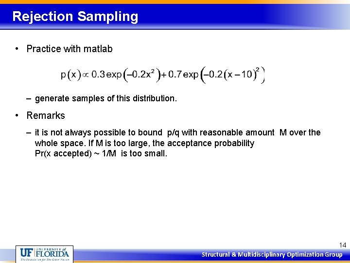
Rejection Sampling • Practice with matlab – generate samples of this distribution. • Remarks – it is not always possible to bound p/q with reasonable amount M over the whole space. If M is too large, the acceptance probability Pr(x accepted) ~ 1/M is too small. 14 Structural & Multidisciplinary Optimization Group

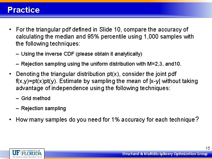
Practice • For the triangular pdf defined in Slide 10, compare the accuracy of calculating the median and 95% percentile using 1, 000 samples with the following techniques: – Using the inverse CDF (please obtain it analytically) – Rejection sampling using the uniform distribution with M=2, 3, and 10. • Denoting the triangular distribution pt(x), consider the joint pdf f(x, y)=pt(x)pt(y). Estimate by sampling the mean of |x-y| without taking advantage of independence using the following techniques: – Grid method – Rejection sampling • How many samples do you need for 1% accuracy for each technique? 15 Structural & Multidisciplinary Optimization Group