Lecture 10 Parallel Databases Wednesday December 1 st

Lecture 10: Parallel Databases Wednesday, December 1 st, 2010 Dan Suciu -- CSEP 544 Fall 2010 1

Announcements • Take-home Final: this weekend • Next Wednesday: last homework due at midnight (Pig Latin) • Also next Wednesday: last lecture (data provenance, data privacy) Dan Suciu -- CSEP 544 Fall 2010 2

Reading Assignment: “Rethinking the Contract” • What is today’s contract with the optimizer ? • What are the main limitations in today’s optimizers ? • What is a “plan diagram” ? Dan Suciu -- CSEP 544 Fall 2010 3

Overview of Today’s Lecture • Parallel databases (Chapter 22. 1 – 22. 5) • Map/reduce • Pig-Latin – Some slides from Alan Gates (Yahoo!Research) – Mini-tutorial on the slides – Read manual for HW 7 • Bloom filters – Use slides extensively ! – Bloom joins are mentioned on pp. 746 in the book Dan Suciu -- CSEP 544 Fall 2010 4

Parallel v. s. Distributed Databases • Parallel database system: – Improve performance through parallel implementation – Will discuss in class (and are on the final) • Distributed database system: – Data is stored across several sites, each site managed by a DBMS capable of running independently – Will not discuss in class Dan Suciu -- CSEP 544 Fall 2010 5

Parallel DBMSs • Goal – Improve performance by executing multiple operations in parallel • Key benefit – Cheaper to scale than relying on a single increasingly more powerful processor • Key challenge – Ensure overhead and contention do not kill performance Dan Suciu -- CSEP 544 Fall 2010 6

Performance Metrics for Parallel DBMSs • Speedup – More processors higher speed – Individual queries should run faster – Should do more transactions per second (TPS) • Scaleup – More processors can process more data – Batch scaleup • Same query on larger input data should take the same time – Transaction scaleup • N-times as many TPS on N-times larger database • But each transaction typically remains small Dan Suciu -- CSEP 544 Fall 2010 7

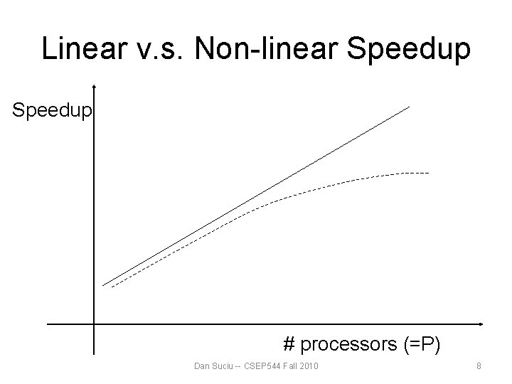
Linear v. s. Non-linear Speedup # processors (=P) Dan Suciu -- CSEP 544 Fall 2010 8

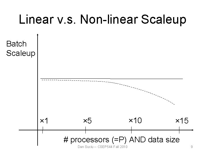
Linear v. s. Non-linear Scaleup Batch Scaleup × 1 × 5 × 10 × 15 # processors (=P) AND data size Dan Suciu -- CSEP 544 Fall 2010 9

Challenges to Linear Speedup and Scaleup • Startup cost – Cost of starting an operation on many processors • Interference – Contention for resources between processors • Skew – Slowest processor becomes the bottleneck Dan Suciu -- CSEP 544 Fall 2010 10

Architectures for Parallel Databases • Shared memory • Shared disk • Shared nothing Dan Suciu -- CSEP 544 Fall 2010 11

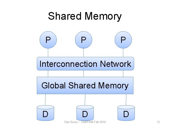
Shared Memory P P P Interconnection Network Global Shared Memory D D Dan Suciu -- CSEP 544 Fall 2010 D 12

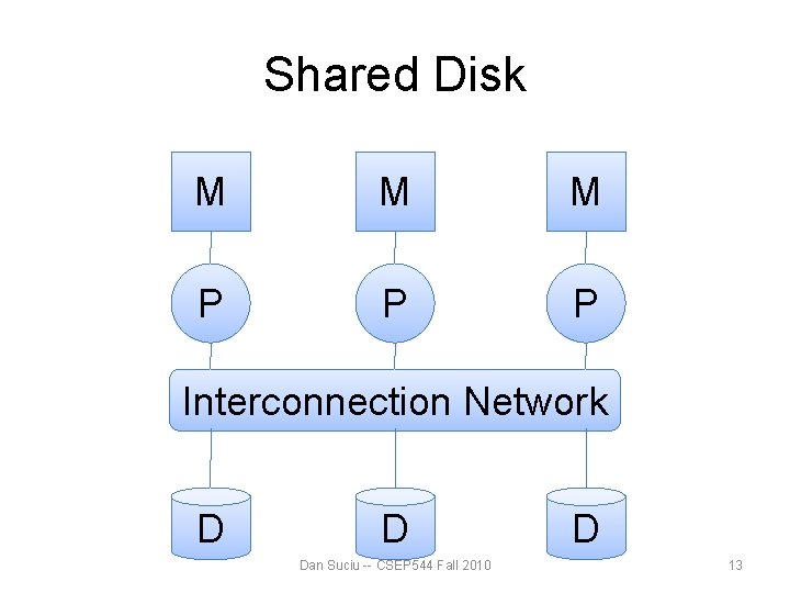
Shared Disk M M M P P P Interconnection Network D D Dan Suciu -- CSEP 544 Fall 2010 D 13

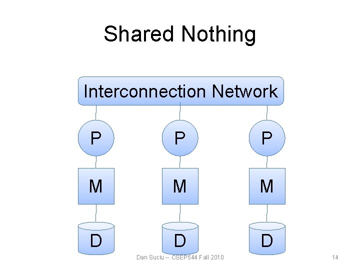
Shared Nothing Interconnection Network P P P M M M D Dan Suciu -- CSEP 544 Fall 2010 14

Shared Nothing • Most scalable architecture – Minimizes interference by minimizing resource sharing – Can use commodity hardware • Also most difficult to program and manage • Processor = server = node • P = number of nodes We will focus on shared nothing Dan Suciu -- CSEP 544 Fall 2010 15

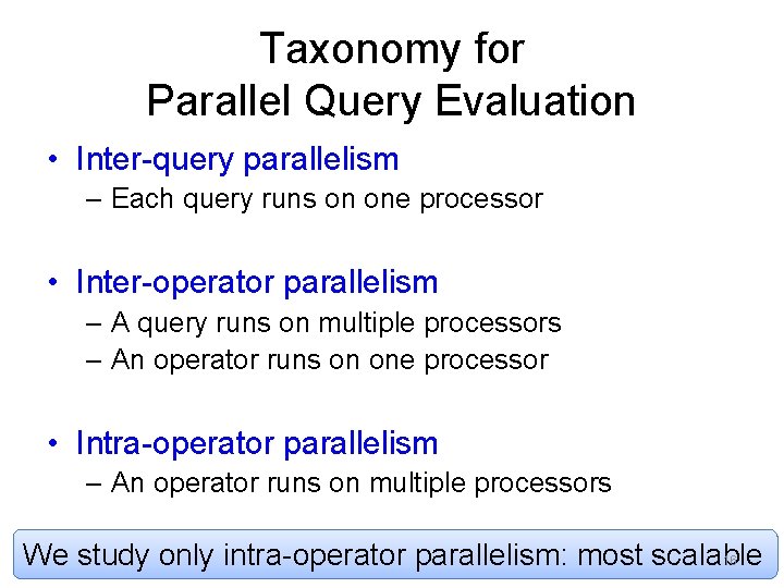
Taxonomy for Parallel Query Evaluation • Inter-query parallelism – Each query runs on one processor • Inter-operator parallelism – A query runs on multiple processors – An operator runs on one processor • Intra-operator parallelism – An operator runs on multiple processors We study only intra-operator parallelism: most scalable Dan Suciu -- CSEP 544 Fall 2010 16

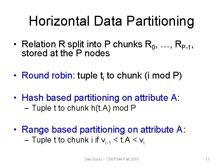
Horizontal Data Partitioning • Relation R split into P chunks R 0, …, RP-1, stored at the P nodes • Round robin: tuple ti to chunk (i mod P) • Hash based partitioning on attribute A: – Tuple t to chunk h(t. A) mod P • Range based partitioning on attribute A: – Tuple t to chunk i if vi-1 < t. A < vi Dan Suciu -- CSEP 544 Fall 2010 17

Parallel Selection Compute σA=v(R), or σv 1<A<v 2(R) • Conventional database: – Cost = B(R) • Parallel database with P processors: – Cost = B(R) / P Dan Suciu -- CSEP 544 Fall 2010 18

Parallel Selection Different processors do the work: • Round robin partition: all servers do the work • Hash partition: – One server for σA=v(R), – All servers for σv 1<A<v 2(R) • Range partition: one server does the work Dan Suciu -- CSEP 544 Fall 2010 19

Data Partitioning Revisited What are the pros and cons ? • Round robin – Good load balance but always needs to read all the data • Hash based partitioning – Good load balance but works only for equality predicates and full scans • Range based partitioning – Works well for range predicates but can suffer from data skew Dan Suciu -- CSEP 544 Fall 2010 20

Parallel Group By: γA, sum(B)(R) Step 1: server i partitions chunk Ri using a hash function h(t. A): Ri 0, Ri 1, …, Ri, P-1 Step 2: server i sends partition Rij to server j Step 3: server j computes γA, sum(B) on R 0 j, R 1 j, …, RP-1, j Dan Suciu -- CSEP 544 Fall 2010 21

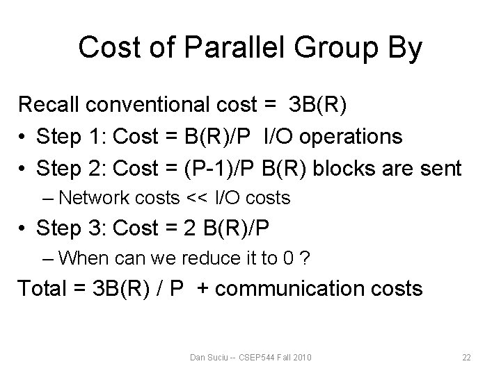
Cost of Parallel Group By Recall conventional cost = 3 B(R) • Step 1: Cost = B(R)/P I/O operations • Step 2: Cost = (P-1)/P B(R) blocks are sent – Network costs << I/O costs • Step 3: Cost = 2 B(R)/P – When can we reduce it to 0 ? Total = 3 B(R) / P + communication costs Dan Suciu -- CSEP 544 Fall 2010 22

Parallel Join: R ⋈A=B S Step 1 • For all servers in [0, k], server i partitions chunk Ri using a hash function h(t. A): Ri 0, Ri 1, …, Ri, P-1 • For all servers in [k+1, P], server j partitions chunk Sj using a hash function h(t. A): Sj 0, Sj 1, …, Rj, P-1 Step 2: • Server i sends partition Riu to server u • Server j sends partition Sju to server u Steps 3: Server u computes the join of Riu with Sju Dan Suciu -- CSEP 544 Fall 2010 23

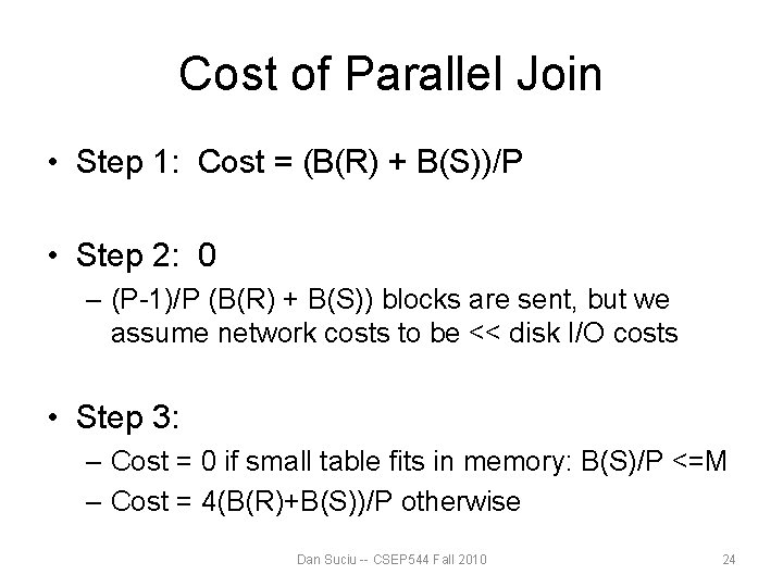
Cost of Parallel Join • Step 1: Cost = (B(R) + B(S))/P • Step 2: 0 – (P-1)/P (B(R) + B(S)) blocks are sent, but we assume network costs to be << disk I/O costs • Step 3: – Cost = 0 if small table fits in memory: B(S)/P <=M – Cost = 4(B(R)+B(S))/P otherwise Dan Suciu -- CSEP 544 Fall 2010 24

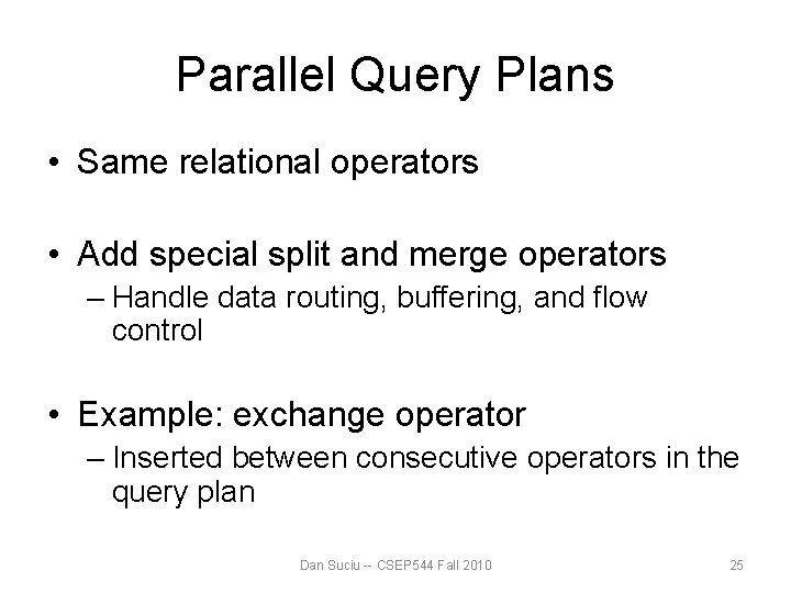
Parallel Query Plans • Same relational operators • Add special split and merge operators – Handle data routing, buffering, and flow control • Example: exchange operator – Inserted between consecutive operators in the query plan Dan Suciu -- CSEP 544 Fall 2010 25

Map Reduce • Google: paper published 2004 • Free variant: Hadoop • Map-reduce = high-level programming model and implementation for large-scale parallel data processing Dan Suciu -- CSEP 544 Fall 2010 26

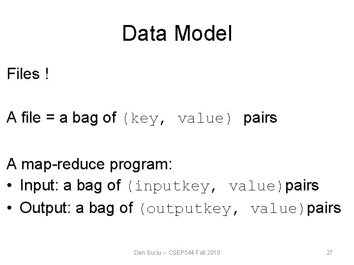
Data Model Files ! A file = a bag of (key, value) pairs A map-reduce program: • Input: a bag of (inputkey, value)pairs • Output: a bag of (outputkey, value)pairs Dan Suciu -- CSEP 544 Fall 2010 27

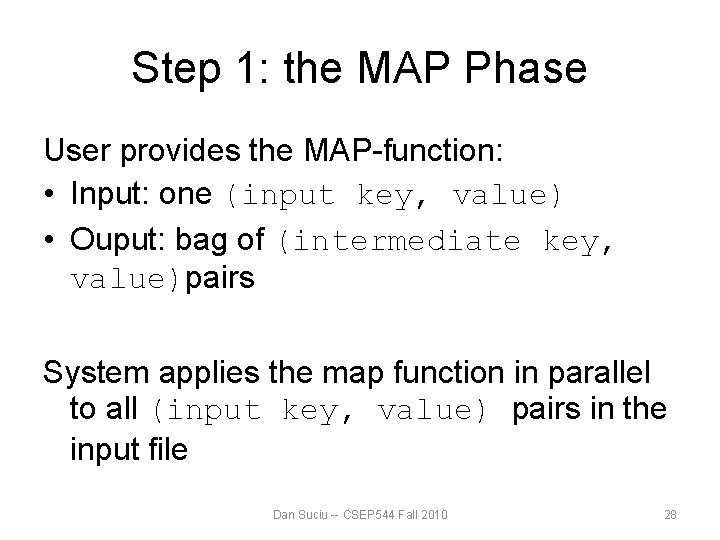
Step 1: the MAP Phase User provides the MAP-function: • Input: one (input key, value) • Ouput: bag of (intermediate key, value)pairs System applies the map function in parallel to all (input key, value) pairs in the input file Dan Suciu -- CSEP 544 Fall 2010 28

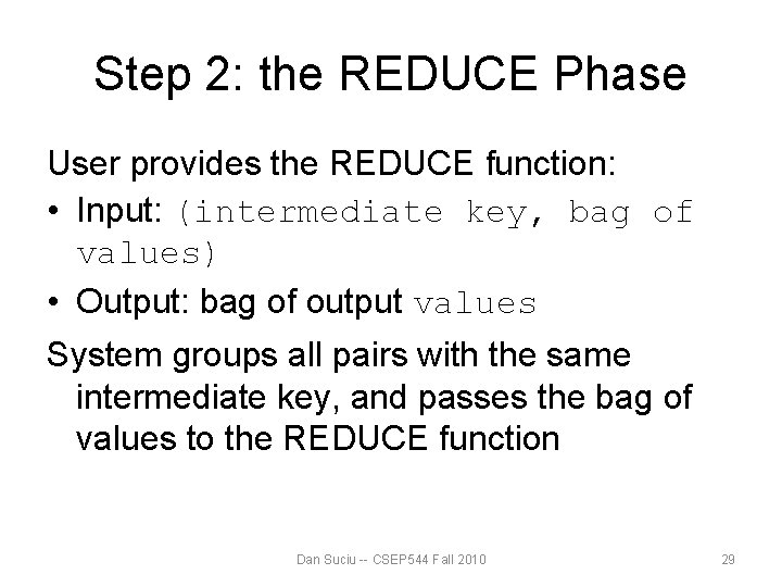
Step 2: the REDUCE Phase User provides the REDUCE function: • Input: (intermediate key, bag of values) • Output: bag of output values System groups all pairs with the same intermediate key, and passes the bag of values to the REDUCE function Dan Suciu -- CSEP 544 Fall 2010 29

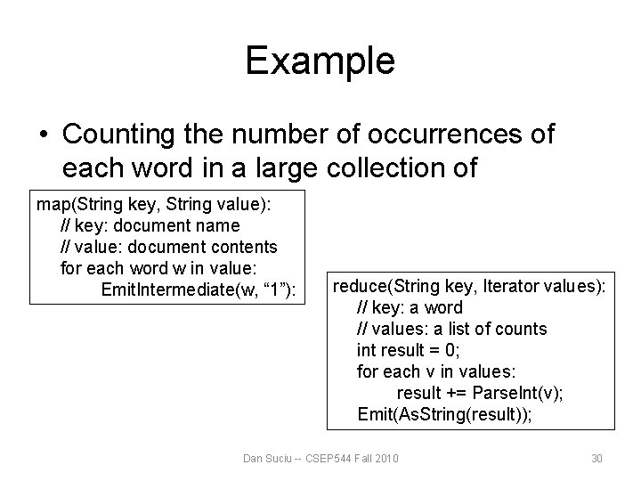
Example • Counting the number of occurrences of each word in a large collection of map(String key, String value): documents // key: document name // value: document contents for each word w in value: Emit. Intermediate(w, “ 1”): reduce(String key, Iterator values): // key: a word // values: a list of counts int result = 0; for each v in values: result += Parse. Int(v); Emit(As. String(result)); Dan Suciu -- CSEP 544 Fall 2010 30

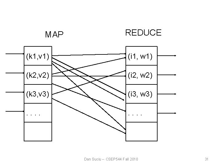
MAP REDUCE (k 1, v 1) (i 1, w 1) (k 2, v 2) (i 2, w 2) (k 3, v 3) (i 3, w 3) . . . . Dan Suciu -- CSEP 544 Fall 2010 31

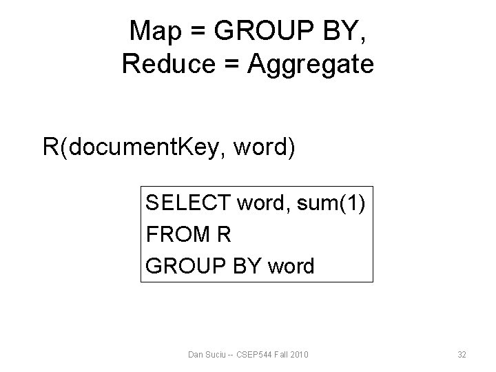
Map = GROUP BY, Reduce = Aggregate R(document. Key, word) SELECT word, sum(1) FROM R GROUP BY word Dan Suciu -- CSEP 544 Fall 2010 32

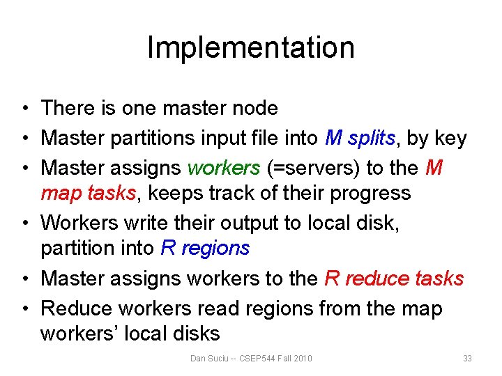
Implementation • There is one master node • Master partitions input file into M splits, by key • Master assigns workers (=servers) to the M map tasks, keeps track of their progress • Workers write their output to local disk, partition into R regions • Master assigns workers to the R reduce tasks • Reduce workers read regions from the map workers’ local disks Dan Suciu -- CSEP 544 Fall 2010 33

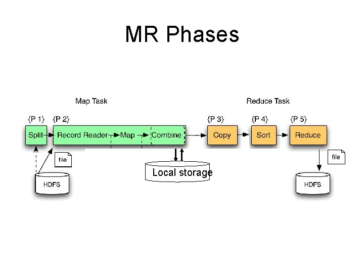
MR Phases Local`storage

Interesting Implementation Details • Worker failure: – Master pings workers periodically, – If down then reassigns its splits to all other workers good load balance • Choice of M and R: – Larger is better for load balancing – Limitation: master needs O(M×R) memory Dan Suciu -- CSEP 544 Fall 2010 35

Interesting Implementation Details Backup tasks: • Straggler = a machine that takes unusually long time to complete one of the last tasks. Eg: – Bad disk forces frequent correctable errors (30 MB/s 1 MB/s) – The cluster scheduler has scheduled other tasks on that machine • Stragglers are a main reason for slowdown • Solution: pre-emptive backup execution of the last few remaining in-progress tasks Dan Suciu -- CSEP 544 Fall 2010 36

Map-Reduce Summary • Hides scheduling and parallelization details • However, very limited queries – Difficult to write more complex tasks – Need multiple map-reduce operations • Solution: PIG-Latin ! Dan Suciu -- CSEP 544 Fall 2010 37

Following Slides provided by: Alan Gates, Yahoo!Research Dan Suciu -- CSEP 544 Fall 2010 38

What is Pig? • An engine for executing programs on top of Hadoop • It provides a language, Pig Latin, to specify these programs • An Apache open source project http: //hadoop. apache. org/pig/ - 39 -

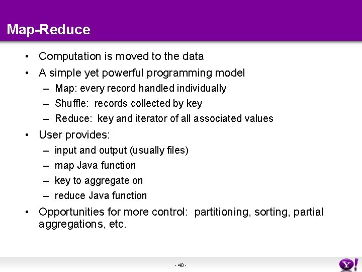
Map-Reduce • Computation is moved to the data • A simple yet powerful programming model – Map: every record handled individually – Shuffle: records collected by key – Reduce: key and iterator of all associated values • User provides: – – input and output (usually files) map Java function key to aggregate on reduce Java function • Opportunities for more control: partitioning, sorting, partial aggregations, etc. - 40 -

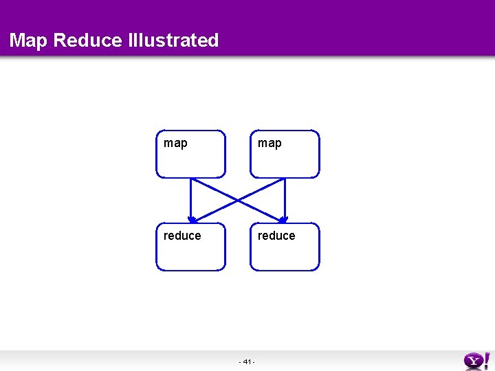
Map Reduce Illustrated map reduce - 41 -

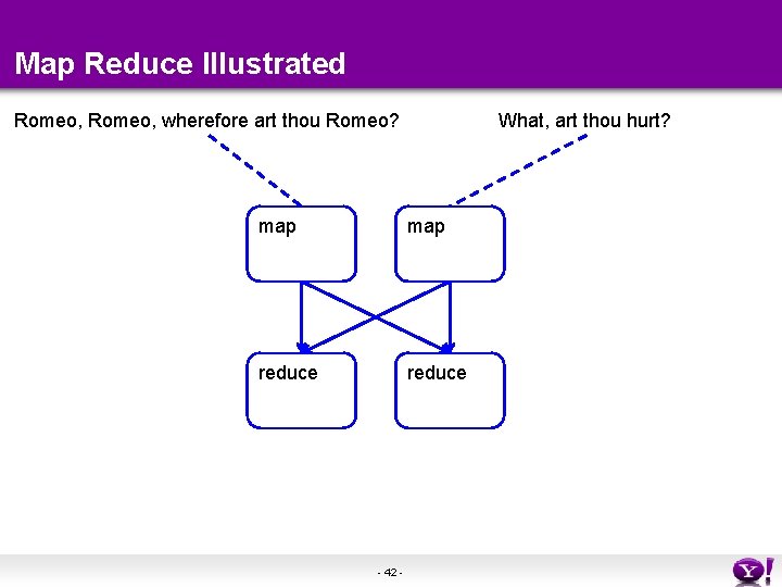
Map Reduce Illustrated Romeo, wherefore art thou Romeo? What, art thou hurt? map reduce - 42 -

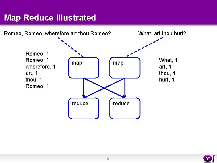
Map Reduce Illustrated Romeo, wherefore art thou Romeo? Romeo, 1 wherefore, 1 art, 1 thou, 1 Romeo, 1 What, art thou hurt? map reduce - 43 - What, 1 art, 1 thou, 1 hurt, 1

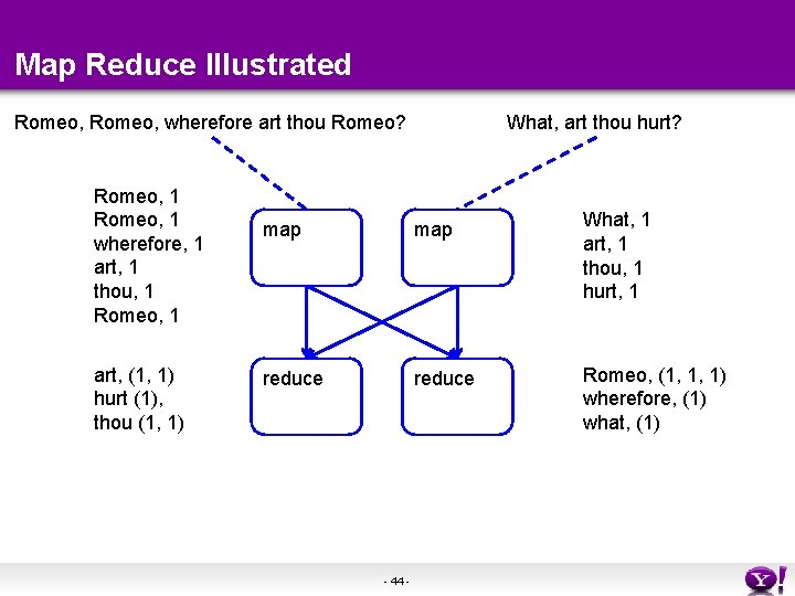
Map Reduce Illustrated Romeo, wherefore art thou Romeo? Romeo, 1 wherefore, 1 art, 1 thou, 1 Romeo, 1 art, (1, 1) hurt (1), thou (1, 1) What, art thou hurt? map What, 1 art, 1 thou, 1 hurt, 1 reduce Romeo, (1, 1, 1) wherefore, (1) what, (1) - 44 -

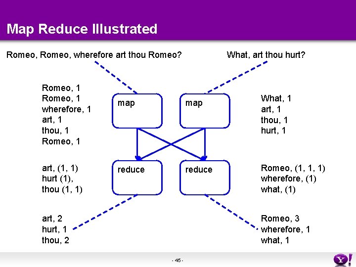
Map Reduce Illustrated Romeo, wherefore art thou Romeo? Romeo, 1 wherefore, 1 art, 1 thou, 1 Romeo, 1 art, (1, 1) hurt (1), thou (1, 1) What, art thou hurt? map What, 1 art, 1 thou, 1 hurt, 1 reduce Romeo, (1, 1, 1) wherefore, (1) what, (1) art, 2 hurt, 1 thou, 2 Romeo, 3 wherefore, 1 what, 1 - 45 -

Making Parallelism Simple • Sequential reads = good read speeds • In large cluster failures are guaranteed; Map Reduce handles retries • Good fit for batch processing applications that need to touch all your data: – data mining – model tuning • Bad fit for applications that need to find one particular record • Bad fit for applications that need to communicate between processes; oriented around independent units of work - 46 -

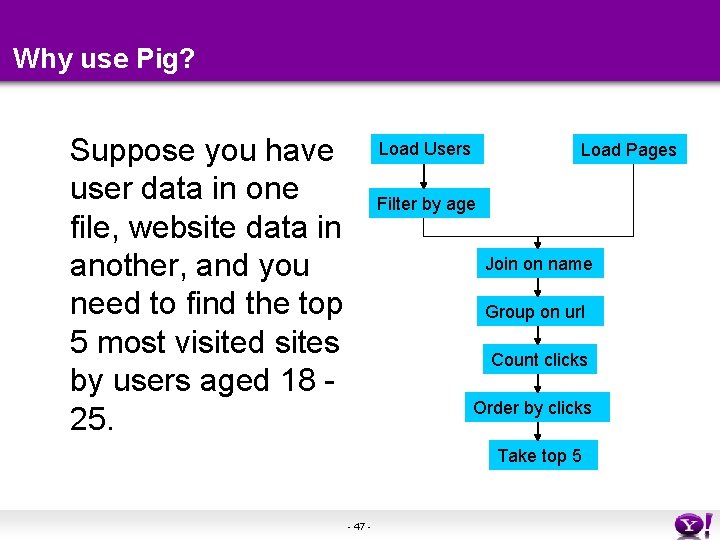
Why use Pig? Suppose you have user data in one file, website data in another, and you need to find the top 5 most visited sites by users aged 18 25. Load Users Load Pages Filter by age Join on name Group on url Count clicks Order by clicks Take top 5 - 47 -

In Map-Reduce 170 lines of code, 4 hours to write - 48 -

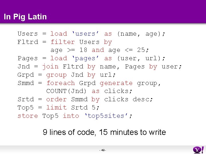
In Pig Latin Users = load ‘users’ as (name, age); Fltrd = filter Users by age >= 18 and age <= 25; Pages = load ‘pages’ as (user, url); Jnd = join Fltrd by name, Pages by user; Grpd = group Jnd by url; Smmd = foreach Grpd generate group, COUNT(Jnd) as clicks; Srtd = order Smmd by clicks desc; Top 5 = limit Srtd 5; store Top 5 into ‘top 5 sites’; 9 lines of code, 15 minutes to write - 49 -

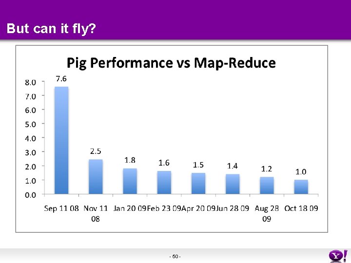
But can it fly? - 50 -

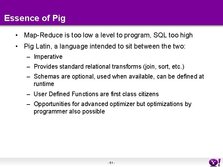
Essence of Pig • Map-Reduce is too low a level to program, SQL too high • Pig Latin, a language intended to sit between the two: – Imperative – Provides standard relational transforms (join, sort, etc. ) – Schemas are optional, used when available, can be defined at runtime – User Defined Functions are first class citizens – Opportunities for advanced optimizer but optimizations by programmer also possible - 51 -

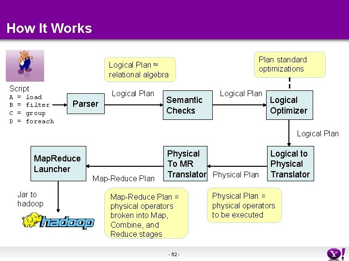
How It Works Plan standard optimizations Logical Plan ≈ relational algebra Script A B C D = = load filter group foreach Logical Plan Parser Semantic Checks Logical Plan Logical Optimizer Logical Plan Map. Reduce Launcher Map-Reduce Plan Jar to hadoop Physical To MR Translator Physical Plan Map-Reduce Plan = physical operators broken into Map, Combine, and Reduce stages - 52 - Logical to Physical Translator Physical Plan = physical operators to be executed

Cool Things We’ve Added In the Last Year • Multiquery – Ability to combine multiple group bys into a single MR job (0. 3) • Merge join – If data is already sorted on join key, do join via merge in map phase (0. 4) • Skew join – Hash join for data with skew in join key. Allows splitting of key across multiple reducers to handle skew. (0. 4) • Zebra – Contrib project that provides columnar storage of data (0. 4) • Rework of Load and Store functions to make them much easier to write (0. 7, branched but not released) • Owl, a metadata service for the grid (committed, will be released in 0. 8). - 53 -

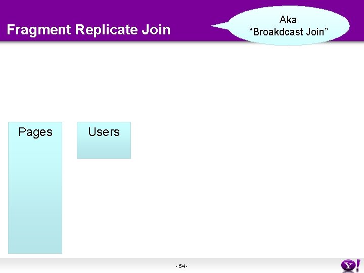
Aka “Broakdcast Join” Fragment Replicate Join Pages Users - 54 -

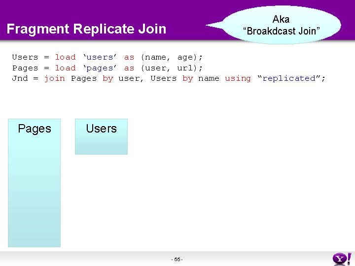
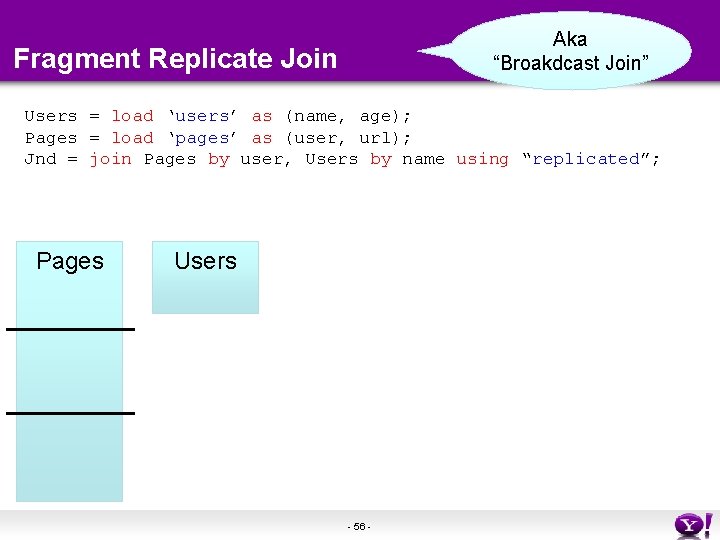
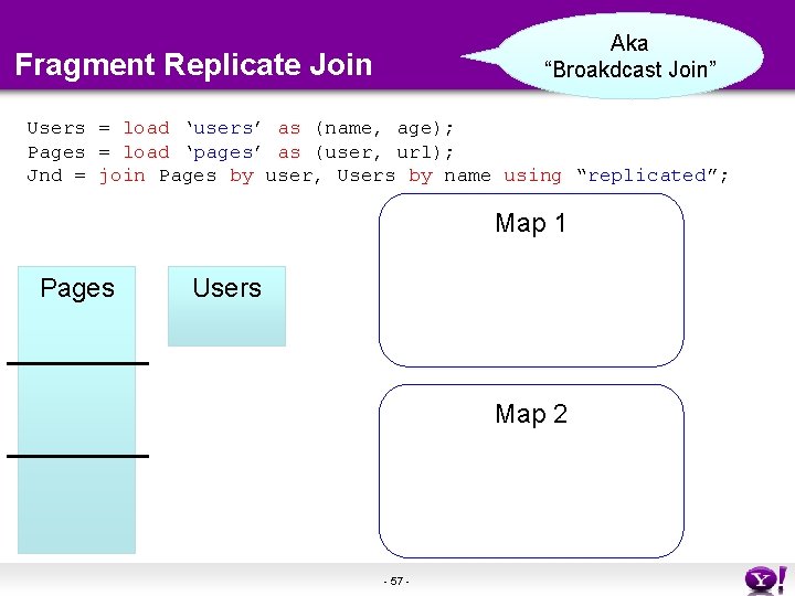
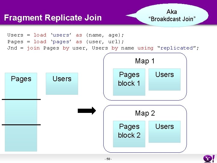
Aka “Broakdcast Join” Fragment Replicate Join Users = load ‘users’ as (name, age); Pages = load ‘pages’ as (user, url); Jnd = join Pages by user, Users by name using “replicated”; Pages Users - 55 -

Aka “Broakdcast Join” Fragment Replicate Join Users = load ‘users’ as (name, age); Pages = load ‘pages’ as (user, url); Jnd = join Pages by user, Users by name using “replicated”; Pages Users - 56 -

Aka “Broakdcast Join” Fragment Replicate Join Users = load ‘users’ as (name, age); Pages = load ‘pages’ as (user, url); Jnd = join Pages by user, Users by name using “replicated”; Map 1 Pages Users Map 2 - 57 -

Aka “Broakdcast Join” Fragment Replicate Join Users = load ‘users’ as (name, age); Pages = load ‘pages’ as (user, url); Jnd = join Pages by user, Users by name using “replicated”; Map 1 Pages block 1 Users Map 2 Pages block 2 - 58 - Users

Hash Join Pages Users - 59 -

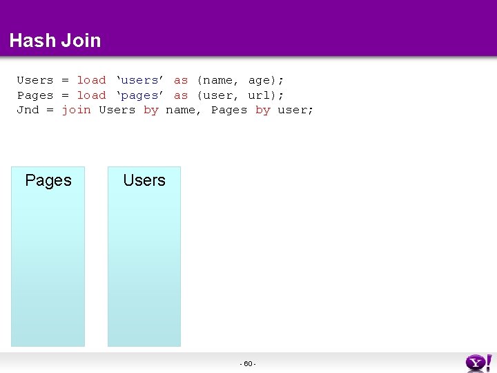
Hash Join Users = load ‘users’ as (name, age); Pages = load ‘pages’ as (user, url); Jnd = join Users by name, Pages by user; Pages Users - 60 -

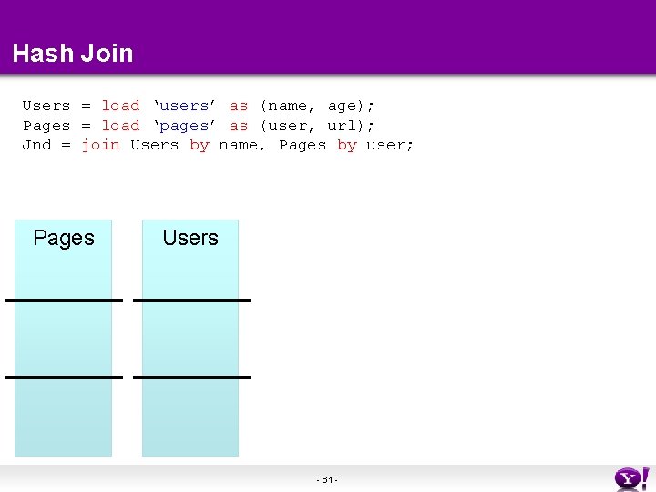
Hash Join Users = load ‘users’ as (name, age); Pages = load ‘pages’ as (user, url); Jnd = join Users by name, Pages by user; Pages Users - 61 -

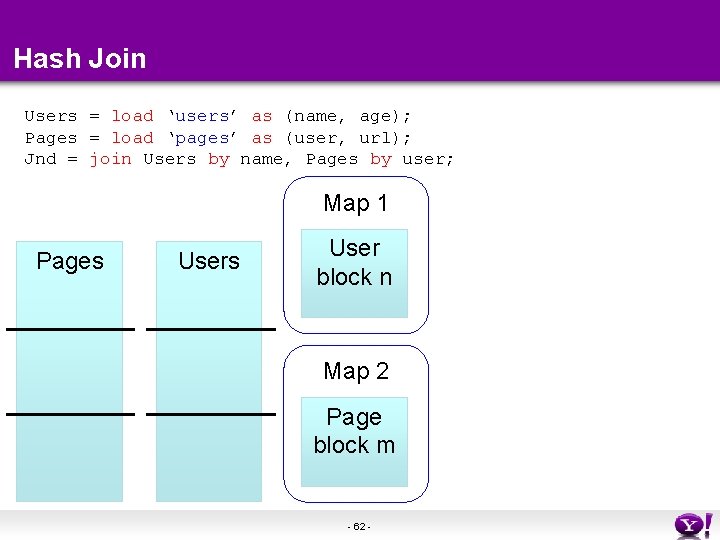
Hash Join Users = load ‘users’ as (name, age); Pages = load ‘pages’ as (user, url); Jnd = join Users by name, Pages by user; Map 1 Pages User block n Map 2 Page block m - 62 -

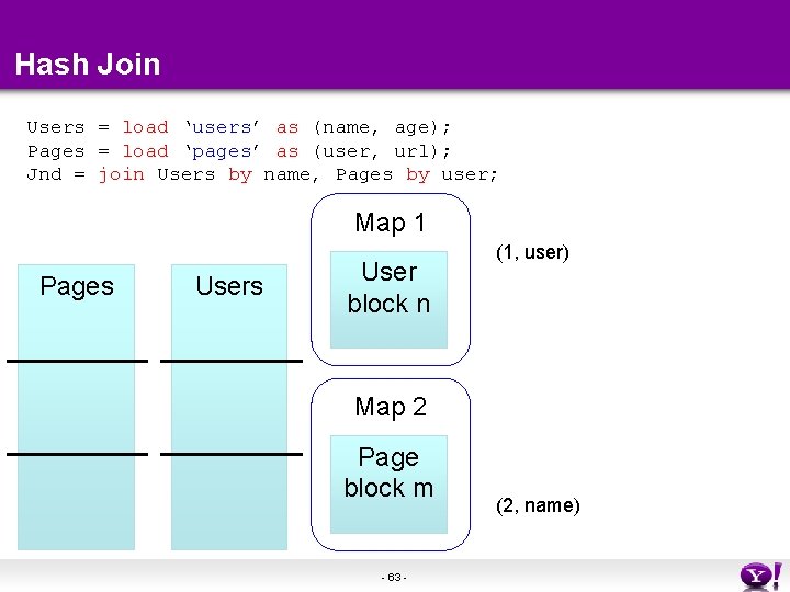
Hash Join Users = load ‘users’ as (name, age); Pages = load ‘pages’ as (user, url); Jnd = join Users by name, Pages by user; Map 1 Pages User block n (1, user) Map 2 Page block m - 63 - (2, name)

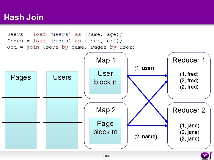
Hash Join Users = load ‘users’ as (name, age); Pages = load ‘pages’ as (user, url); Jnd = join Users by name, Pages by user; Map 1 Pages User block n Reducer 1 (1, user) Map 2 Page block m - 64 - (1, fred) (2, fred) Reducer 2 (2, name) (1, jane) (2, jane)

Skew Join Pages Users - 65 -

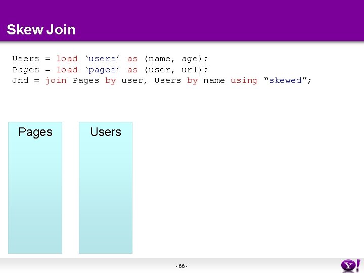
Skew Join Users = load ‘users’ as (name, age); Pages = load ‘pages’ as (user, url); Jnd = join Pages by user, Users by name using “skewed”; Pages Users - 66 -

Skew Join Users = load ‘users’ as (name, age); Pages = load ‘pages’ as (user, url); Jnd = join Pages by user, Users by name using “skewed”; Pages Users - 67 -

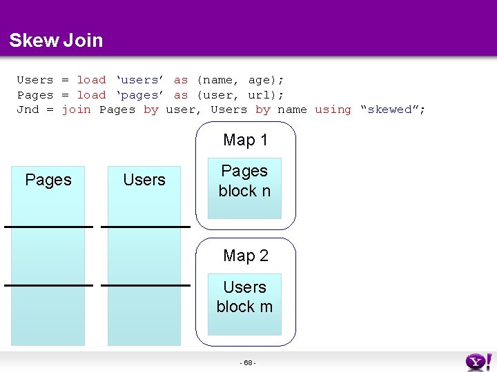
Skew Join Users = load ‘users’ as (name, age); Pages = load ‘pages’ as (user, url); Jnd = join Pages by user, Users by name using “skewed”; Map 1 Pages Users Pages block n Map 2 Users block m - 68 -

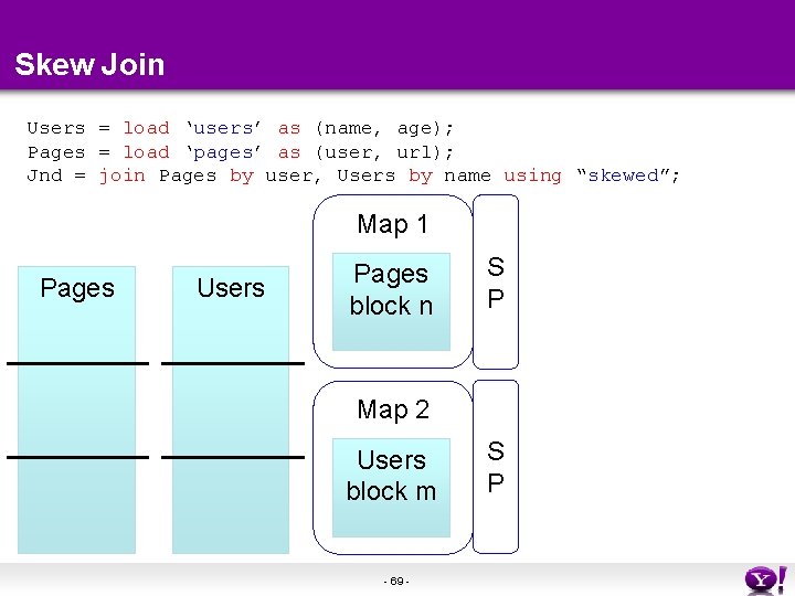
Skew Join Users = load ‘users’ as (name, age); Pages = load ‘pages’ as (user, url); Jnd = join Pages by user, Users by name using “skewed”; Map 1 Pages Users Pages block n S P Map 2 Users block m - 69 - S P

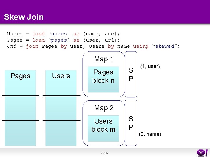
Skew Join Users = load ‘users’ as (name, age); Pages = load ‘pages’ as (user, url); Jnd = join Pages by user, Users by name using “skewed”; Map 1 Pages Users Pages block n S P (1, user) Map 2 Users block m - 70 - S P (2, name)

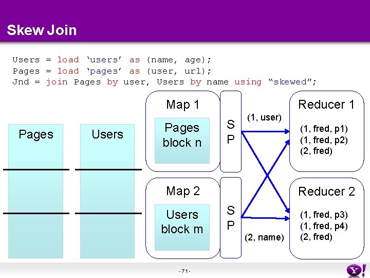
Skew Join Users = load ‘users’ as (name, age); Pages = load ‘pages’ as (user, url); Jnd = join Pages by user, Users by name using “skewed”; Map 1 Pages Users Pages block n Reducer 1 S P (1, user) (1, fred, p 1) (1, fred, p 2) (2, fred) Map 2 Users block m - 71 - Reducer 2 S P (2, name) (1, fred, p 3) (1, fred, p 4) (2, fred)

Merge Join Pages Users aaron. . . . zach - 72 -

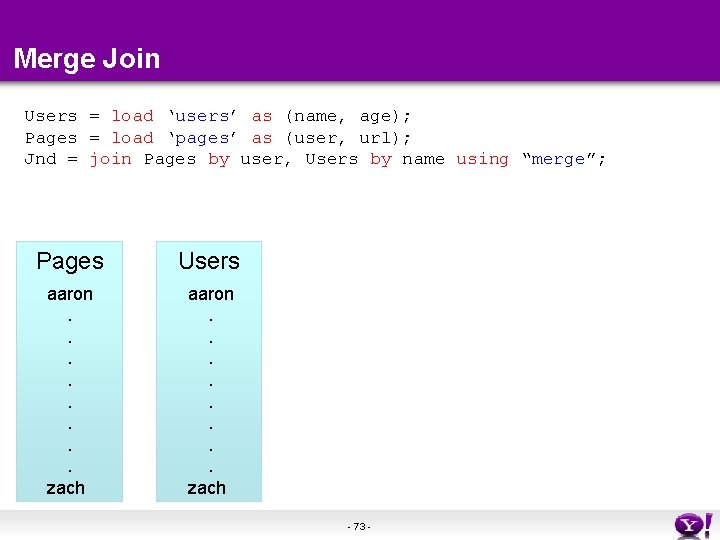
Merge Join Users = load ‘users’ as (name, age); Pages = load ‘pages’ as (user, url); Jnd = join Pages by user, Users by name using “merge”; Pages Users aaron. . . . zach - 73 -

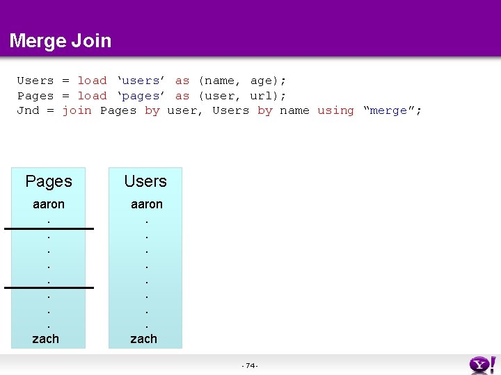
Merge Join Users = load ‘users’ as (name, age); Pages = load ‘pages’ as (user, url); Jnd = join Pages by user, Users by name using “merge”; Pages Users aaron. . . . zach - 74 -

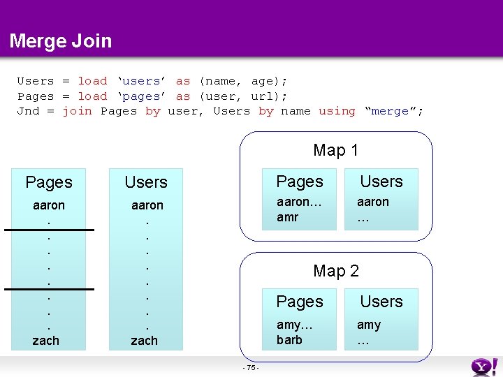
Merge Join Users = load ‘users’ as (name, age); Pages = load ‘pages’ as (user, url); Jnd = join Pages by user, Users by name using “merge”; Map 1 Pages Users aaron. . . . zach aaron… amr aaron … Map 2 - 75 - Pages Users amy… barb amy …

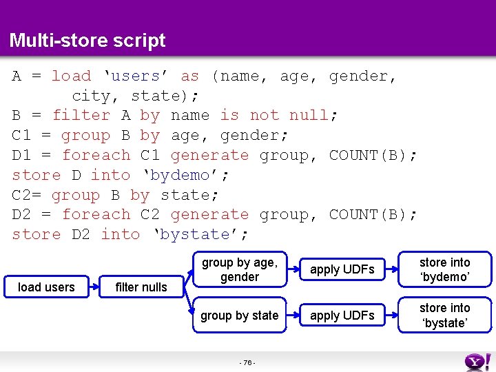
Multi-store script A = load ‘users’ as (name, age, gender, city, state); B = filter A by name is not null; C 1 = group B by age, gender; D 1 = foreach C 1 generate group, COUNT(B); store D into ‘bydemo’; C 2= group B by state; D 2 = foreach C 2 generate group, COUNT(B); store D 2 into ‘bystate’; load users filter nulls group by age, gender apply UDFs store into ‘bydemo’ group by state apply UDFs store into ‘bystate’ - 76 -

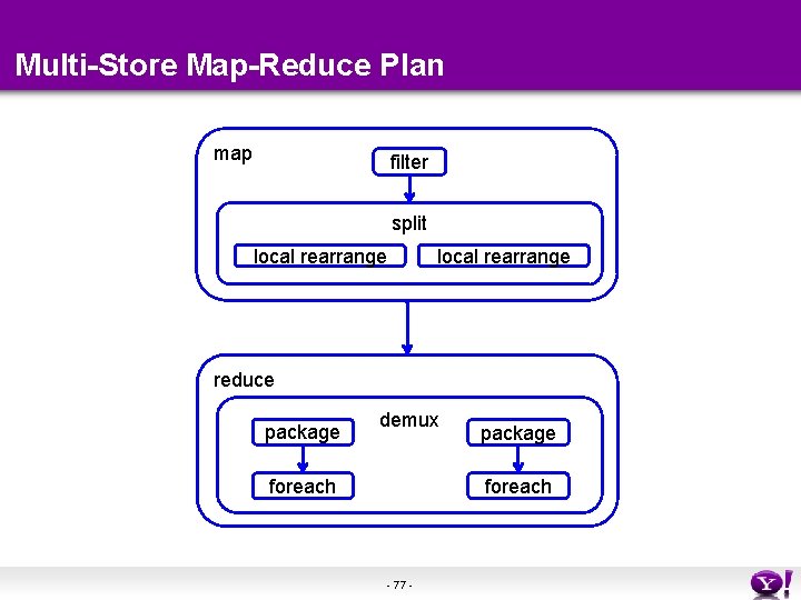
Multi-Store Map-Reduce Plan map filter split local rearrange reduce package demux foreach package foreach - 77 -

What are people doing with Pig • At Yahoo ~70% of Hadoop jobs are Pig jobs • Being used at Twitter, Linked. In, and other companies • Available as part of Amazon EMR web service and Cloudera Hadoop distribution • What users use Pig for: – – – – Search infrastructure Ad relevance Model training User intent analysis Web log processing Image processing Incremental processing of large data sets - 78 -

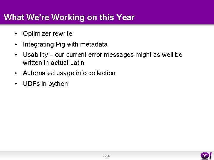
What We’re Working on this Year • Optimizer rewrite • Integrating Pig with metadata • Usability – our current error messages might as well be written in actual Latin • Automated usage info collection • UDFs in python - 79 -

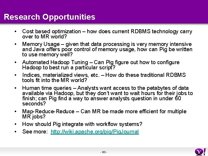
Research Opportunities • • Cost based optimization – how does current RDBMS technology carry over to MR world? Memory Usage – given that data processing is very memory intensive and Java offers poor control of memory usage, how can Pig be written to use memory well? Automated Hadoop Tuning – Can Pig figure out how to configure Hadoop to best run a particular script? Indices, materialized views, etc. – How do these traditional RDBMS tools fit into the MR world? Human time queries – Analysts want access to the petabytes of data available via Hadoop, but they don’t want to wait hours for their jobs to finish; can Pig find a way to answer analysts question in under 60 seconds? Map-Reduce – Can MR be made more efficient for multiple MR jobs? How should Pig integrate with workflow systems? See more: http: //wiki. apache. org/pig/Pig. Journal - 80 -

Learn More • Visit our website: http: //hadoop. apache. org/pig/ • On line tutorials – From Yahoo, http: //developer. yahoo. com/hadoop/tutorial/ – From Cloudera, http: //www. cloudera. com/hadoop-training • A couple of Hadoop books are available that include chapters on Pig, search at your favorite bookstore • Join the mailing lists: – pig-user@hadoop. apache. org for user questions – pig-dev@hadoop. apache. com for developer issues • Contribute your work, over 50 people have so far - 81 -

Pig Latin Mini-Tutorial (will skip in class; please read in order to do homework 7) 82

Outline Based entirely on Pig Latin: A not-soforeign language for data processing, by Olston, Reed, Srivastava, Kumar, and Tomkins, 2008 Quiz section tomorrow: in CSE 403 (this is CSE, don’t go to EE 1) 83

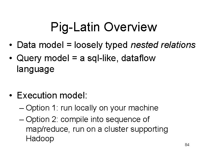
Pig-Latin Overview • Data model = loosely typed nested relations • Query model = a sql-like, dataflow language • Execution model: – Option 1: run locally on your machine – Option 2: compile into sequence of map/reduce, run on a cluster supporting Hadoop 84

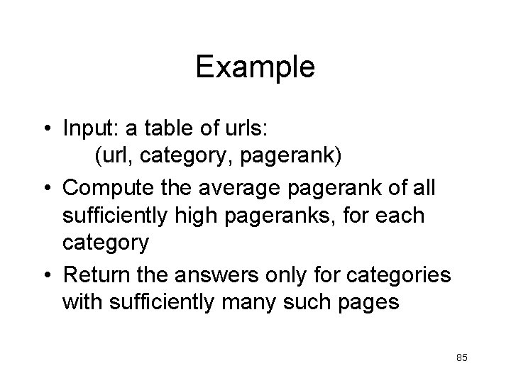
Example • Input: a table of urls: (url, category, pagerank) • Compute the average pagerank of all sufficiently high pageranks, for each category • Return the answers only for categories with sufficiently many such pages 85

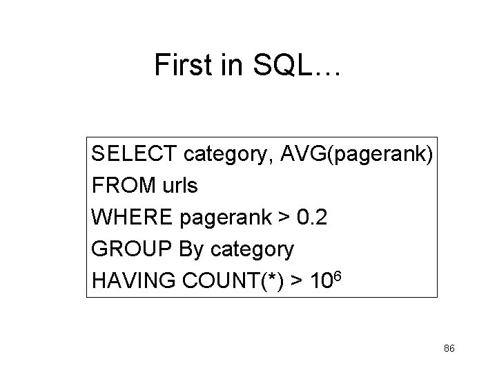
First in SQL… SELECT category, AVG(pagerank) FROM urls WHERE pagerank > 0. 2 GROUP By category HAVING COUNT(*) > 106 86

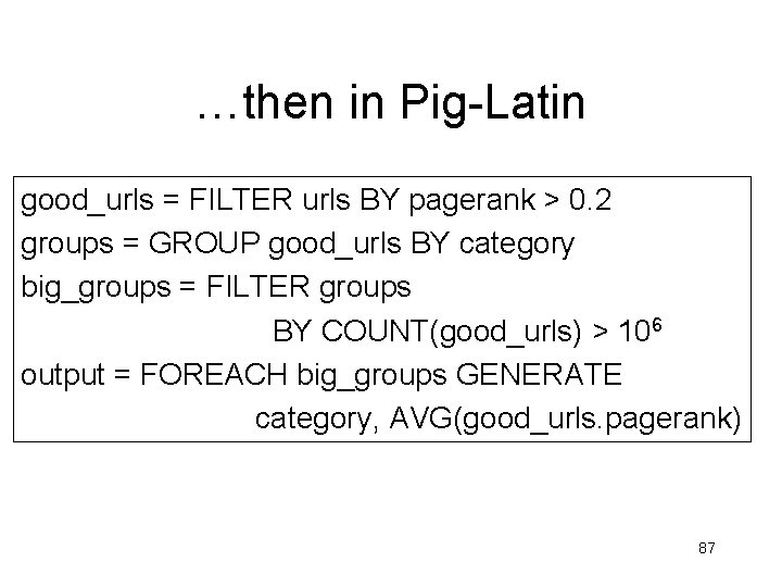
…then in Pig-Latin good_urls = FILTER urls BY pagerank > 0. 2 groups = GROUP good_urls BY category big_groups = FILTER groups BY COUNT(good_urls) > 106 output = FOREACH big_groups GENERATE category, AVG(good_urls. pagerank) 87

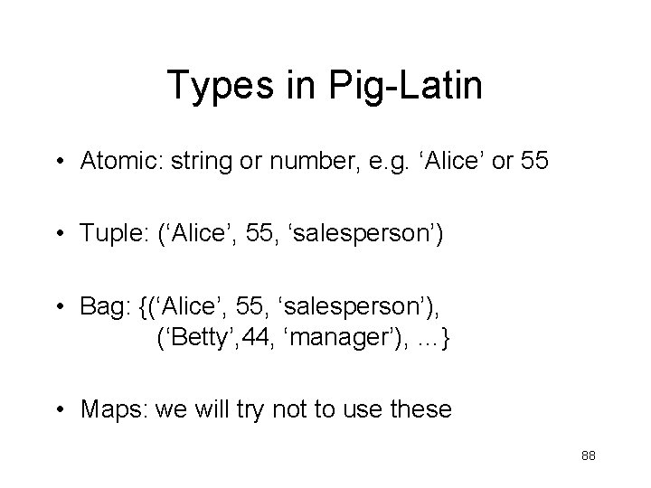
Types in Pig-Latin • Atomic: string or number, e. g. ‘Alice’ or 55 • Tuple: (‘Alice’, 55, ‘salesperson’) • Bag: {(‘Alice’, 55, ‘salesperson’), (‘Betty’, 44, ‘manager’), …} • Maps: we will try not to use these 88

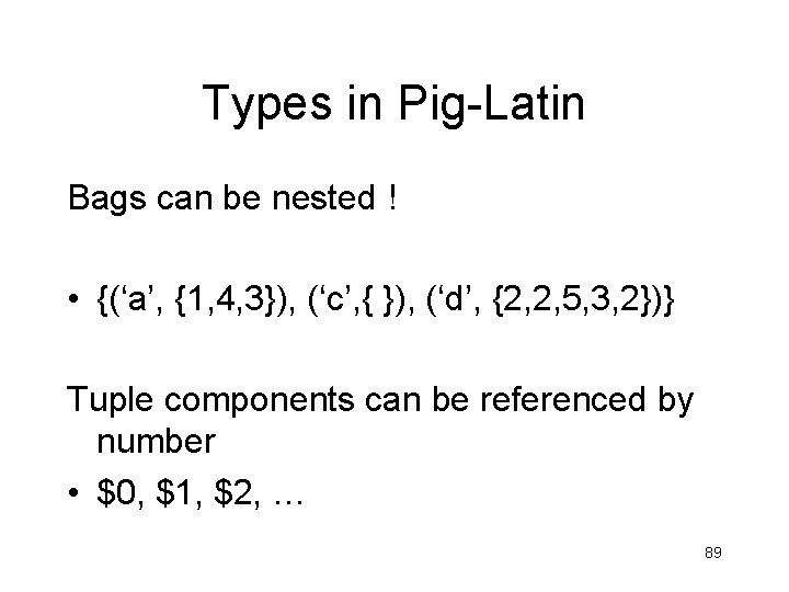
Types in Pig-Latin Bags can be nested ! • {(‘a’, {1, 4, 3}), (‘c’, { }), (‘d’, {2, 2, 5, 3, 2})} Tuple components can be referenced by number • $0, $1, $2, … 89

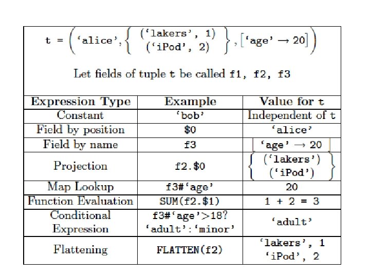
90

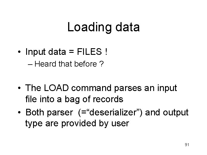
Loading data • Input data = FILES ! – Heard that before ? • The LOAD command parses an input file into a bag of records • Both parser (=“deserializer”) and output type are provided by user 91

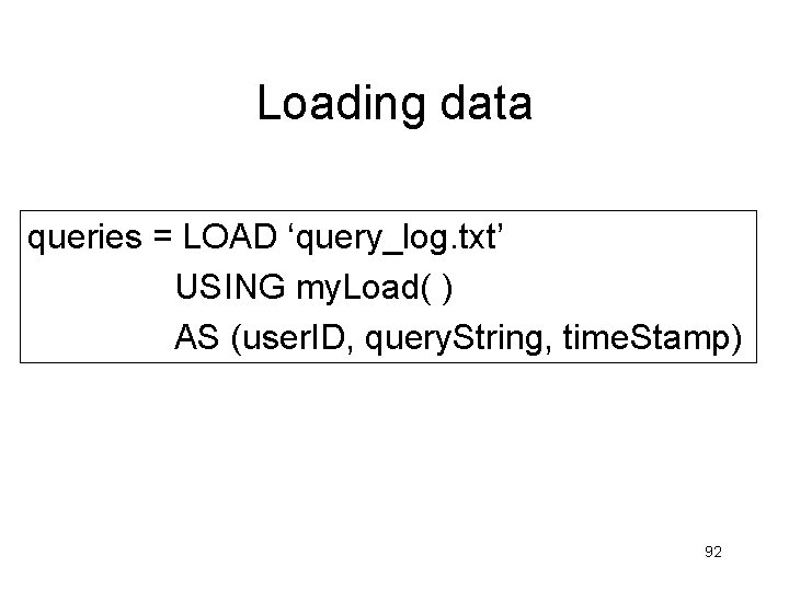
Loading data queries = LOAD ‘query_log. txt’ USING my. Load( ) AS (user. ID, query. String, time. Stamp) 92

Loading data • USING userfuction( ) -- is optional – Default deserializer expects tab-delimited file • AS type – is optional – Default is a record with unnamed fields; refer to them as $0, $1, … • The return value of LOAD is just a handle to a bag – The actual reading is done in pull mode, or parallelized 93

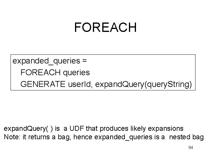
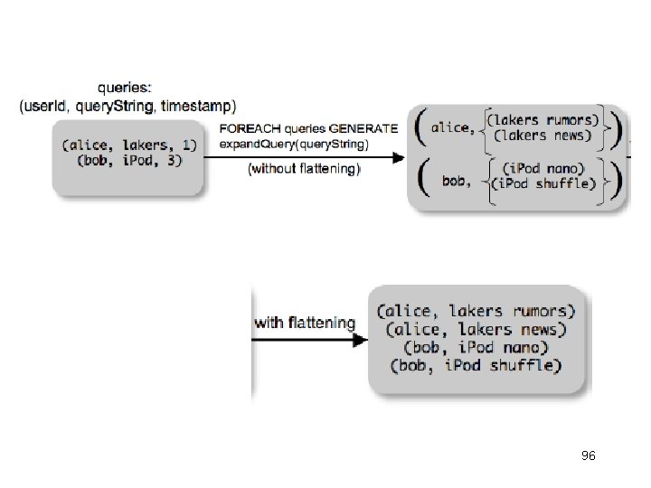
FOREACH expanded_queries = FOREACH queries GENERATE user. Id, expand. Query(query. String) expand. Query( ) is a UDF that produces likely expansions Note: it returns a bag, hence expanded_queries is a nested bag 94

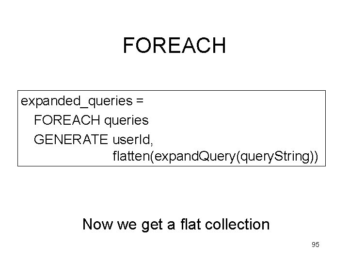
FOREACH expanded_queries = FOREACH queries GENERATE user. Id, flatten(expand. Query(query. String)) Now we get a flat collection 95

96

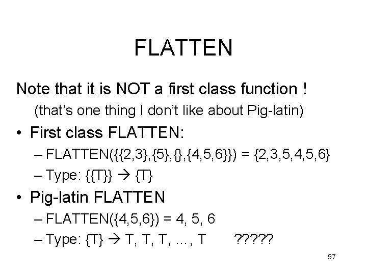
FLATTEN Note that it is NOT a first class function ! (that’s one thing I don’t like about Pig-latin) • First class FLATTEN: – FLATTEN({{2, 3}, {5}, {4, 5, 6}}) = {2, 3, 5, 4, 5, 6} – Type: {{T}} {T} • Pig-latin FLATTEN – FLATTEN({4, 5, 6}) = 4, 5, 6 – Type: {T} T, T, T, …, T ? ? ? 97

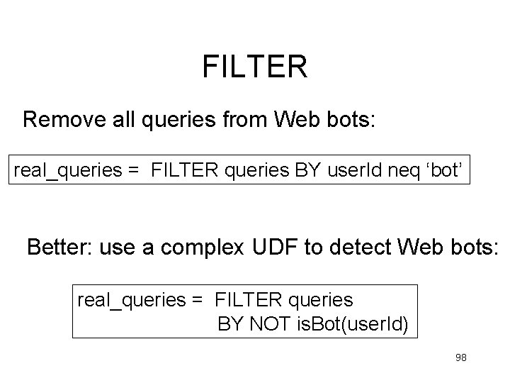
FILTER Remove all queries from Web bots: real_queries = FILTER queries BY user. Id neq ‘bot’ Better: use a complex UDF to detect Web bots: real_queries = FILTER queries BY NOT is. Bot(user. Id) 98

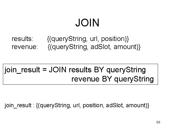
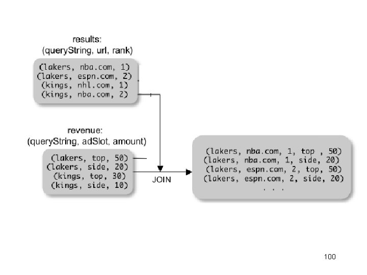
JOIN results: revenue: {(query. String, url, position)} {(query. String, ad. Slot, amount)} join_result = JOIN results BY query. String revenue BY query. String join_result : {(query. String, url, position, ad. Slot, amount)} 99

100

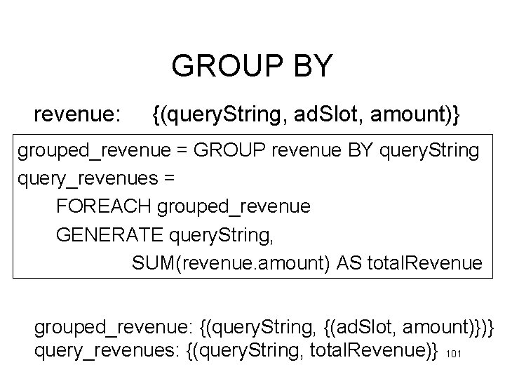
GROUP BY revenue: {(query. String, ad. Slot, amount)} grouped_revenue = GROUP revenue BY query. String query_revenues = FOREACH grouped_revenue GENERATE query. String, SUM(revenue. amount) AS total. Revenue grouped_revenue: {(query. String, {(ad. Slot, amount)})} query_revenues: {(query. String, total. Revenue)} 101

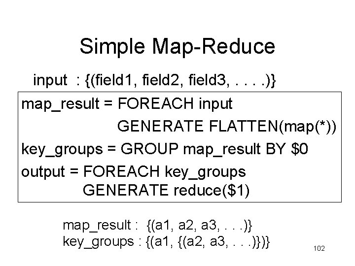
Simple Map-Reduce input : {(field 1, field 2, field 3, . . )} map_result = FOREACH input GENERATE FLATTEN(map(*)) key_groups = GROUP map_result BY $0 output = FOREACH key_groups GENERATE reduce($1) map_result : {(a 1, a 2, a 3, . . . )} key_groups : {(a 1, {(a 2, a 3, . . . )})} 102

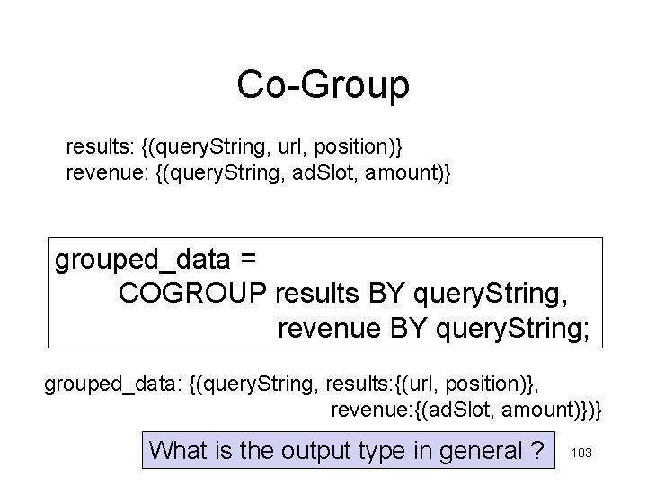
Co-Group results: {(query. String, url, position)} revenue: {(query. String, ad. Slot, amount)} grouped_data = COGROUP results BY query. String, revenue BY query. String; grouped_data: {(query. String, results: {(url, position)}, revenue: {(ad. Slot, amount)})} What is the output type in general ? 103

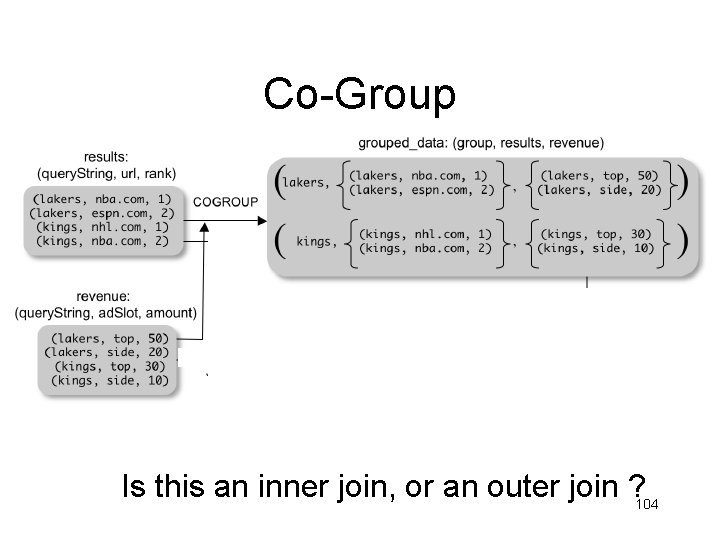
Co-Group Is this an inner join, or an outer join ? 104

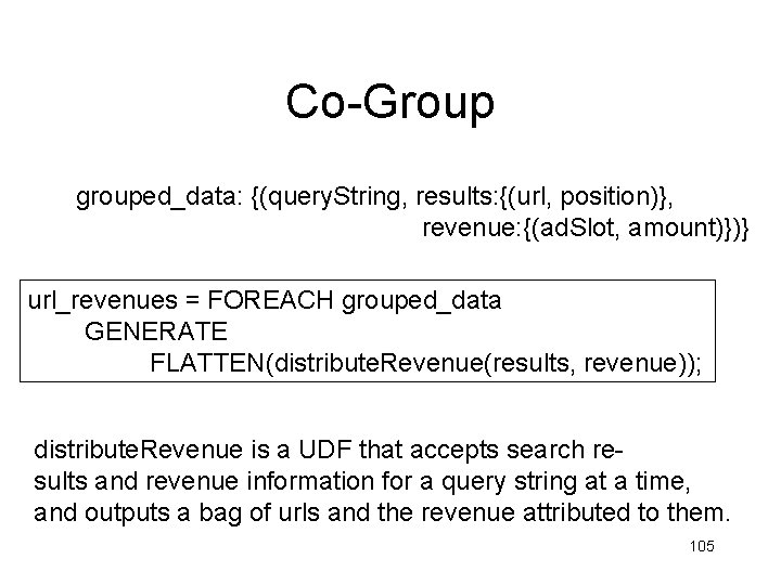
Co-Group grouped_data: {(query. String, results: {(url, position)}, revenue: {(ad. Slot, amount)})} url_revenues = FOREACH grouped_data GENERATE FLATTEN(distribute. Revenue(results, revenue)); distribute. Revenue is a UDF that accepts search results and revenue information for a query string at a time, and outputs a bag of urls and the revenue attributed to them. 105

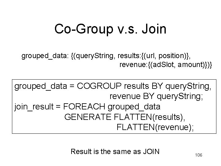
Co-Group v. s. Join grouped_data: {(query. String, results: {(url, position)}, revenue: {(ad. Slot, amount)})} grouped_data = COGROUP results BY query. String, revenue BY query. String; join_result = FOREACH grouped_data GENERATE FLATTEN(results), FLATTEN(revenue); Result is the same as JOIN 106

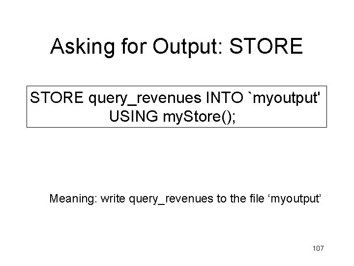
Asking for Output: STORE query_revenues INTO `myoutput' USING my. Store(); Meaning: write query_revenues to the file ‘myoutput’ 107

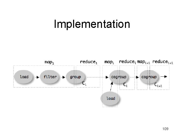
Implementation • Over Hadoop ! • Parse query: – Everything between LOAD and STORE one logical plan • Logical plan sequence of Map/Reduce ops • All statements between two (CO)GROUPs one Map/Reduce op 108

Implementation 109

Bloom Filters We *WILL* discuss in class ! Dan Suciu -- CSEP 544 Fall 2010 110

Lecture on Bloom Filters Not described in the textbook ! Lecture based in part on: • Broder, Andrei; Mitzenmacher, Michael (2005), "Network Applications of Bloom Filters: A Survey", Internet Mathematics 1 (4): 485– 509 • Bloom, Burton H. (1970), "Space/time tradeoffs in hash coding with allowable errors", Communications of the ACM 13 (7): 422– 42 Dan Suciu -- CSEP 544 Fall 2010 111

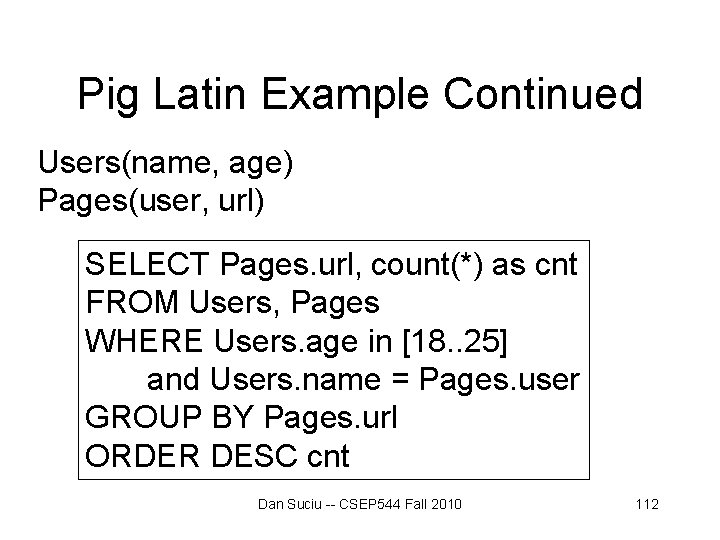
Pig Latin Example Continued Users(name, age) Pages(user, url) SELECT Pages. url, count(*) as cnt FROM Users, Pages WHERE Users. age in [18. . 25] and Users. name = Pages. user GROUP BY Pages. url ORDER DESC cnt Dan Suciu -- CSEP 544 Fall 2010 112

Example Problem: many Pages, but only a few visited by users with age 18. . 25 • Pig’s solution: – MAP phase sends all pages to the reducers • How can we reduce communication cost ? Dan Suciu -- CSEP 544 Fall 2010 113

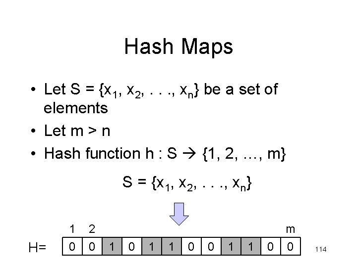
Hash Maps • Let S = {x 1, x 2, . . . , xn} be a set of elements • Let m > n • Hash function h : S {1, 2, …, m} S = {x 1, x 2, . . . , xn} H= 1 0 2 0 1 1 0 0 1 1 m 0 0 114

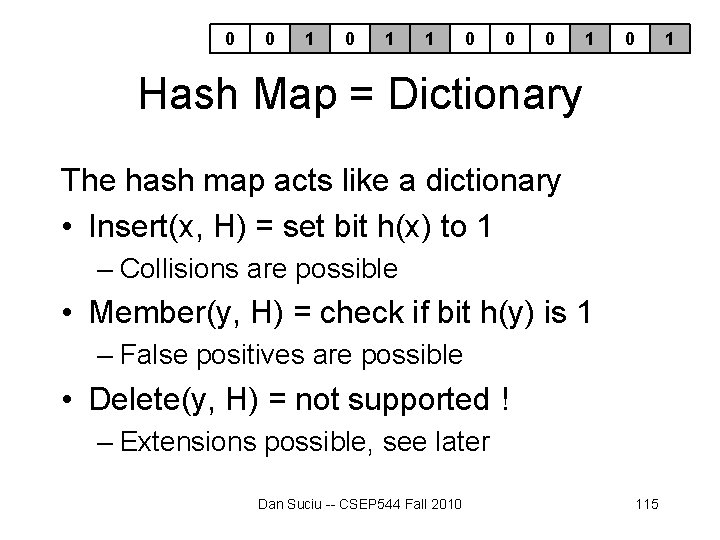
0 0 1 1 0 0 0 1 Hash Map = Dictionary The hash map acts like a dictionary • Insert(x, H) = set bit h(x) to 1 – Collisions are possible • Member(y, H) = check if bit h(y) is 1 – False positives are possible • Delete(y, H) = not supported ! – Extensions possible, see later Dan Suciu -- CSEP 544 Fall 2010 115

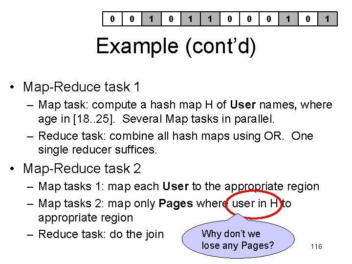
0 0 1 1 0 0 0 1 Example (cont’d) • Map-Reduce task 1 – Map task: compute a hash map H of User names, where age in [18. . 25]. Several Map tasks in parallel. – Reduce task: combine all hash maps using OR. One single reducer suffices. • Map-Reduce task 2 – Map tasks 1: map each User to the appropriate region – Map tasks 2: map only Pages where user in H to appropriate region Why don’t we – Reduce task: do the join lose any Pages? 116

Analysis • Let S = {x 1, x 2, . . . , xn} • Let j = a specific bit in H (1 ≤ j ≤ m) • What is the probability that j remains 0 after inserting all n elements from S into H ? • Will compute in two steps Dan Suciu -- CSEP 544 Fall 2010 117

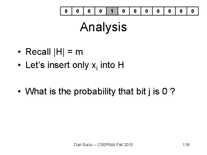
0 0 1 0 0 0 0 Analysis • Recall |H| = m • Let’s insert only xi into H • What is the probability that bit j is 0 ? Dan Suciu -- CSEP 544 Fall 2010 118

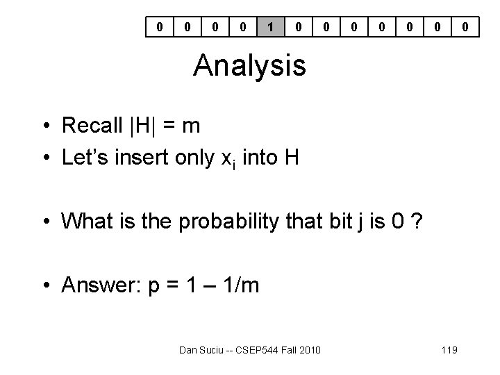
0 0 1 0 0 0 0 Analysis • Recall |H| = m • Let’s insert only xi into H • What is the probability that bit j is 0 ? • Answer: p = 1 – 1/m Dan Suciu -- CSEP 544 Fall 2010 119

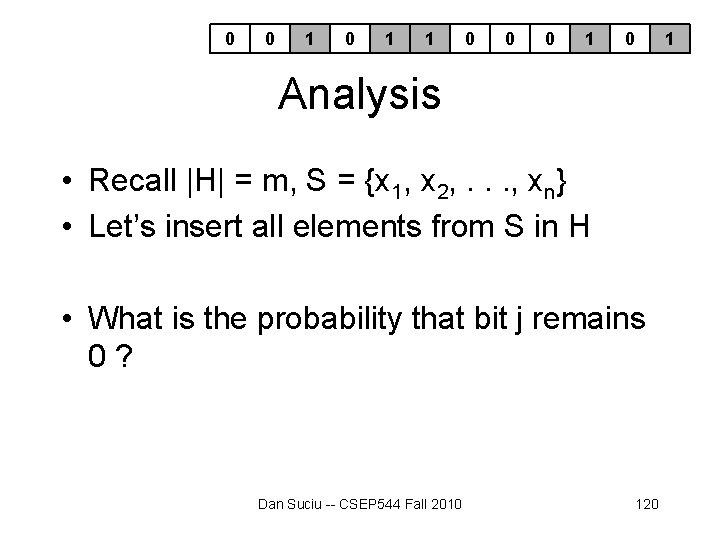
0 0 1 1 0 0 0 1 Analysis • Recall |H| = m, S = {x 1, x 2, . . . , xn} • Let’s insert all elements from S in H • What is the probability that bit j remains 0? Dan Suciu -- CSEP 544 Fall 2010 120

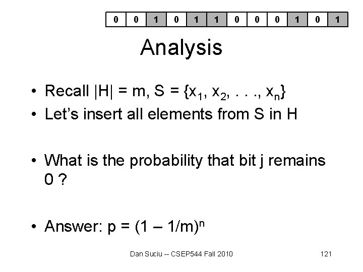
0 0 1 1 0 0 0 1 Analysis • Recall |H| = m, S = {x 1, x 2, . . . , xn} • Let’s insert all elements from S in H • What is the probability that bit j remains 0? • Answer: p = (1 – 1/m)n Dan Suciu -- CSEP 544 Fall 2010 121

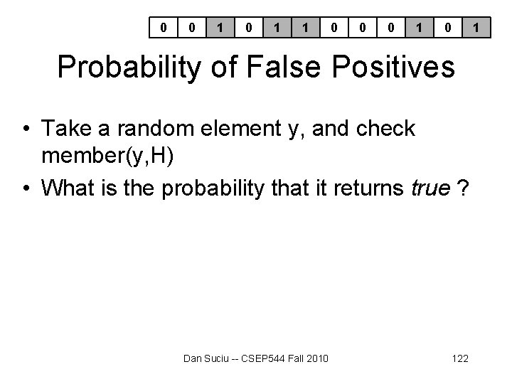
0 0 1 1 0 0 0 1 Probability of False Positives • Take a random element y, and check member(y, H) • What is the probability that it returns true ? Dan Suciu -- CSEP 544 Fall 2010 122

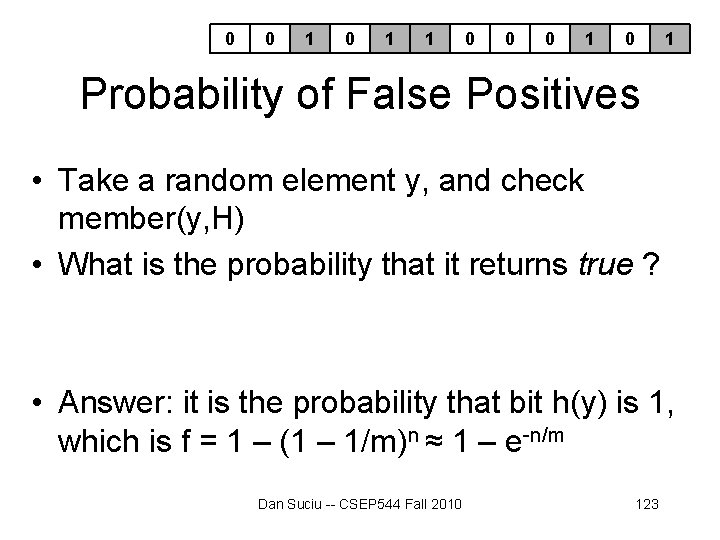
0 0 1 1 0 0 0 1 Probability of False Positives • Take a random element y, and check member(y, H) • What is the probability that it returns true ? • Answer: it is the probability that bit h(y) is 1, which is f = 1 – (1 – 1/m)n ≈ 1 – e-n/m Dan Suciu -- CSEP 544 Fall 2010 123

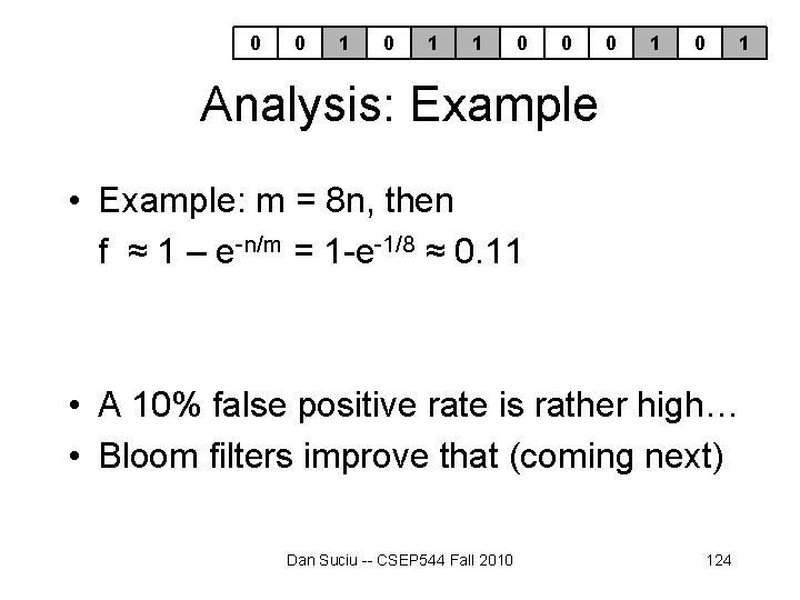
0 0 1 1 0 0 0 1 Analysis: Example • Example: m = 8 n, then f ≈ 1 – e-n/m = 1 -e-1/8 ≈ 0. 11 • A 10% false positive rate is rather high… • Bloom filters improve that (coming next) Dan Suciu -- CSEP 544 Fall 2010 124

Bloom Filters • Introduced by Burton Bloom in 1970 • Improve the false positive ratio • Idea: use k independent hash functions Dan Suciu -- CSEP 544 Fall 2010 125

Bloom Filter = Dictionary • Insert(x, H) = set bits h 1(x), . . . , hk(x) to 1 – Collisions between x and x’ are possible • Member(y, H) = check if bits h 1(y), . . . , hk(y) are 1 – False positives are possible • Delete(z, H) = not supported ! – Extensions possible, see later Dan Suciu -- CSEP 544 Fall 2010 126

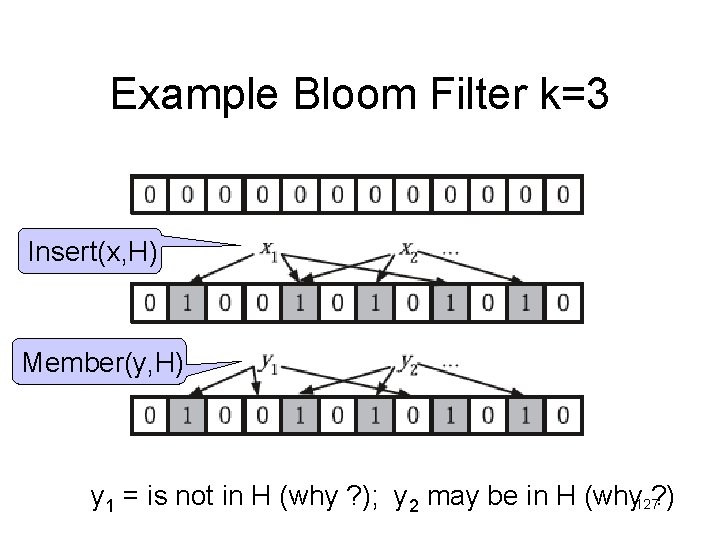
Example Bloom Filter k=3 Insert(x, H) Member(y, H) y 1 = is not in H (why ? ); y 2 may be in H (why 127? )

Choosing k Two competing forces: • If k = large – Test more bits for member(y, H) lower false positive rate – More bits in H are 1 higher false positive rate • If k = small – More bits in H are 0 lower positive rate – Test fewer bits for member(y, H) higher rate Dan Suciu -- CSEP 544 Fall 2010 128

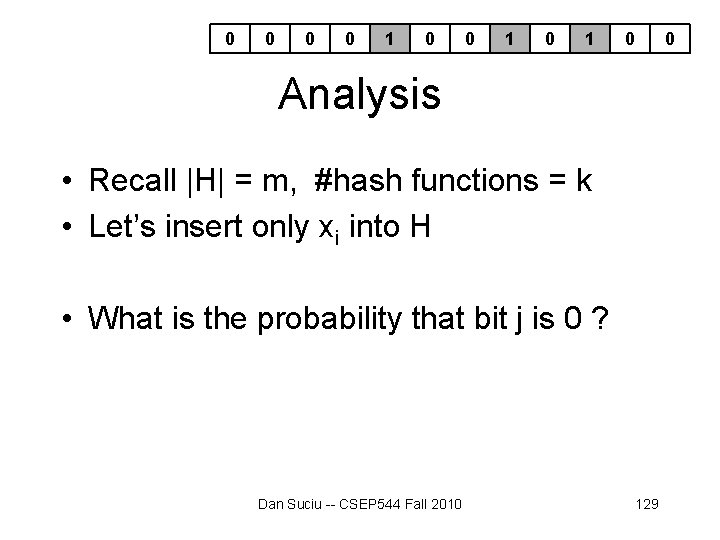
0 0 1 0 0 Analysis • Recall |H| = m, #hash functions = k • Let’s insert only xi into H • What is the probability that bit j is 0 ? Dan Suciu -- CSEP 544 Fall 2010 129

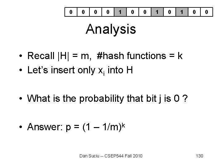
0 0 1 0 0 Analysis • Recall |H| = m, #hash functions = k • Let’s insert only xi into H • What is the probability that bit j is 0 ? • Answer: p = (1 – 1/m)k Dan Suciu -- CSEP 544 Fall 2010 130

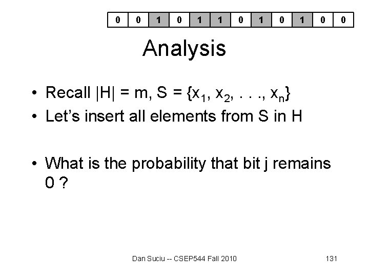
0 0 1 1 0 1 0 0 Analysis • Recall |H| = m, S = {x 1, x 2, . . . , xn} • Let’s insert all elements from S in H • What is the probability that bit j remains 0? Dan Suciu -- CSEP 544 Fall 2010 131

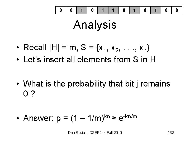
0 0 1 1 0 1 0 0 Analysis • Recall |H| = m, S = {x 1, x 2, . . . , xn} • Let’s insert all elements from S in H • What is the probability that bit j remains 0? • Answer: p = (1 – 1/m)kn ≈ e-kn/m Dan Suciu -- CSEP 544 Fall 2010 132

Probability of False Positives • Take a random element y, and check member(y, H) • What is the probability that it returns true ? Dan Suciu -- CSEP 544 Fall 2010 133

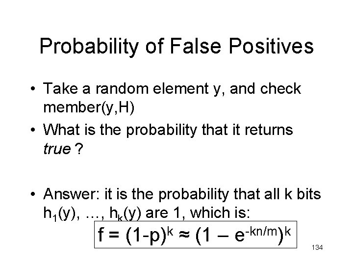
Probability of False Positives • Take a random element y, and check member(y, H) • What is the probability that it returns true ? • Answer: it is the probability that all k bits h 1(y), …, hk(y) are 1, which is: f = (1 -p)k ≈ (1 – e-kn/m)k 134

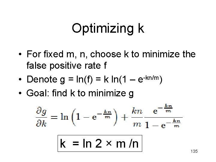
Optimizing k • For fixed m, n, choose k to minimize the false positive rate f • Denote g = ln(f) = k ln(1 – e-kn/m) • Goal: find k to minimize g k = ln 2 × m /n 135

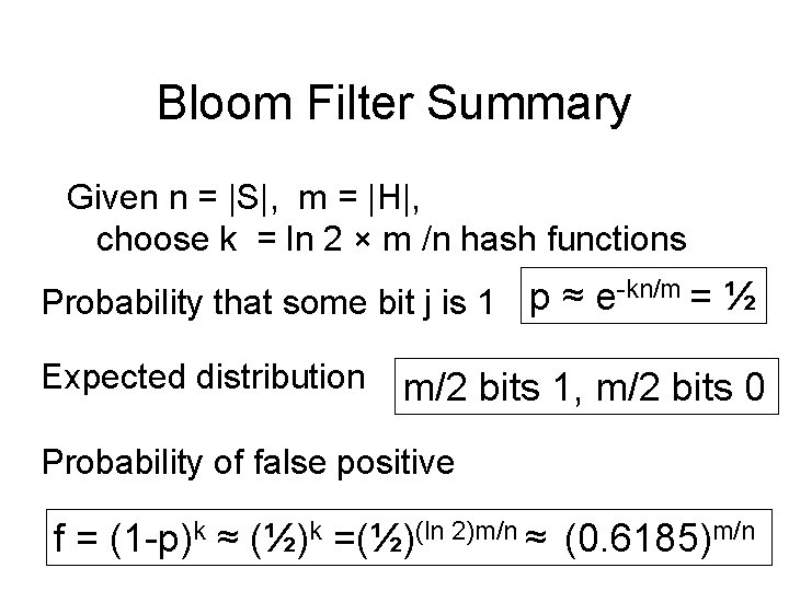
Bloom Filter Summary Given n = |S|, m = |H|, choose k = ln 2 × m /n hash functions Probability that some bit j is 1 p ≈ e-kn/m = ½ Expected distribution m/2 bits 1, m/2 bits 0 Probability of false positive f = (1 -p)k ≈ (½)k =(½)(ln 2)m/n ≈ (0. 6185)m/n 136

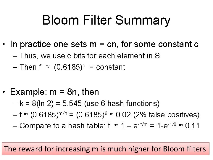
Bloom Filter Summary • In practice one sets m = cn, for some constant c – Thus, we use c bits for each element in S – Then f ≈ (0. 6185)c = constant • Example: m = 8 n, then – k = 8(ln 2) = 5. 545 (use 6 hash functions) – f ≈ (0. 6185)m/n = (0. 6185)8 ≈ 0. 02 (2% false positives) – Compare to a hash table: f ≈ 1 – e-n/m = 1 -e-1/8 ≈ 0. 11 The reward for increasing m is much higher for Bloom filters Dan Suciu -- CSEP 544 Fall 2010 137

Set Operations Intersection and Union of Sets: • Set S Bloom filter H • Set S’ Bloom filter H’ • How do we computed the Bloom filter for the intersection of S and S’ ? Dan Suciu -- CSEP 544 Fall 2010 138

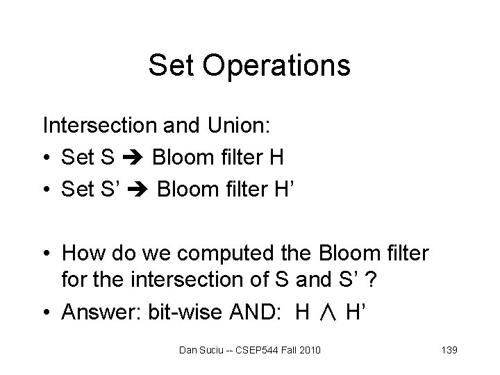
Set Operations Intersection and Union: • Set S Bloom filter H • Set S’ Bloom filter H’ • How do we computed the Bloom filter for the intersection of S and S’ ? • Answer: bit-wise AND: H ∧ H’ Dan Suciu -- CSEP 544 Fall 2010 139

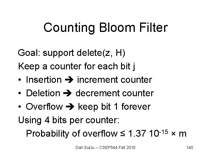
Counting Bloom Filter Goal: support delete(z, H) Keep a counter for each bit j • Insertion increment counter • Deletion decrement counter • Overflow keep bit 1 forever Using 4 bits per counter: Probability of overflow ≤ 1. 37 10 -15 × m Dan Suciu -- CSEP 544 Fall 2010 140

Application: Dictionaries Bloom originally introduced this for hyphenation • 90% of English words can be hyphenated using simple rules • 10% require table lookup • Use “bloom filter” to check if lookup needed Dan Suciu -- CSEP 544 Fall 2010 141

Application: Distributed Caching • Web proxies maintain a cache of (URL, page) pairs • If a URL is not present in the cache, they would like to check the cache of other proxies in the network • Transferring all URLs is expensive ! • Instead: compute Bloom filter, exchange periodically Dan Suciu -- CSEP 544 Fall 2010 142