Lecture 10 Outline Monte Carlo methods n History

Lecture 10 Outline Monte Carlo methods n History of methods n Sequential random number generators n Parallel random number generators n Generating non-uniform random numbers n Monte Carlo case studies n

Monte Carlo Methods n n Monte Carlo is another name for statistical sampling methods of great importance to physics and computer science Applications of Monte Carlo Method u Evaluating integrals of arbitrary functions of 6+ dimensions u Predicting future values of stocks u Solving partial differential equations u Sharpening satellite images u Modeling cell populations u Finding approximate solutions to NP-hard problems

An Interesting History of Statistical Physics • In 1738, Swiss physicist and mathematician Daniel Bernoulli published Hydrodynamica which laid the basis for the kinetic theory of gases: great numbers of molecules moving in all directions, that their impact on a surface causes the gas pressure that we feel, and that we experience as heat is simply the kinetic energy of their motion. • In 1859, Scottish physicist James Clerk Maxwell formulated the distribution of molecular velocities, which gave the proportion of molecules having a certain velocity in a specific range. This was the first -ever statistical law in physics. Maxwell used a simple thought experiment: particles must move independent of any chosen coordinates, hence the only possible distribution of velocities must be normal in each coordinate. • In 1864, Ludwig Boltzmann, a young student in Vienna, came across Maxwell’s paper and was so inspired by it that he spent much of his long, distinguished, and tortured life developing the subject further.

History of Monte Carlo Method n n n Credit for inventing the Monte Carlo method is shared by Stanislaw Ulam, John von Neuman and Nicholas Metropolis. Ulam, a Polish born mathematician, worked for John von Neumann on the Manhattan Project. Ulam is known for designing the hydrogen bomb with Edward Teller in 1951. In a thought experiment he conceived of the MC method in 1946 while pondering the probabilities of winning a card game of solitaire. Ulam, von Neuman, and Metropolis developed algorithms for computer implementations, as well as exploring means of transforming non-random problems into random forms that would facilitate their solution via statistical sampling. This work transformed statistical sampling from a mathematical curiosity to a formal methodology applicable to a wide variety of problems. It was Metropolis who named the new methodology after the casinos of Monte Carlo. Ulam and Metropolis published a paper called “The Monte Carlo Method” in Journal of the American Statistical Association, 44 (247), 335 -341, in 1949.

Errors in Estimation and Two Important Questions for Monte Carlo n n n Errors arise from two sources u Statistical: using finite number of samples to estimate an inifinte sum. u Computational: using finite state machines to produce statistically independent random numbers. Questions u To ensure a level of statistical accuracy, i. e. , m significant digits with probability 1 -1/n, how many samples are needed? u Given n samples, how statistically accurate is the estimate? “the best methods rarely offers more than 2 -3 digit accuracy”-- G. Fishman, Monte Carlo Methods, Springer

Controlling Error n n Two tenets from statistics: u Weak Law of Large Numbers t value of a sum of i. i. d random variables converges to me n u ( u is mean). t So as n grows approx error vanishes u Central Limit Theorem t Sum converges to a normal distribution with mean nu and variance n var sqrt(n) t So as n grows error can be estimated using normal tables and theorems about tails of distribution. Caveats u Convergence rates differ and can be complex u Results in additional error estimates or need larger sample size than normal distribution would indicate

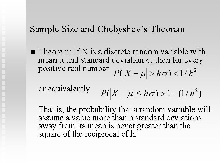
Sample Size and Chebyshev’s Theorem n Theorem: If X is a discrete random variable with mean and standard deviation , then for every positive real number or equivalently That is, the probability that a random variable will assume a value more than h standard deviations away from its mean is never greater than the square of the reciprocal of h.

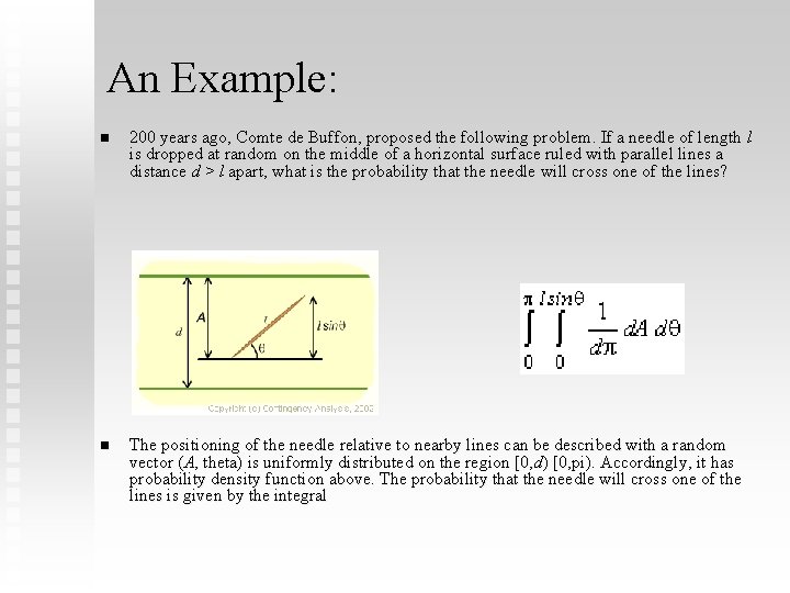
An Example: n 200 years ago, Comte de Buffon, proposed the following problem. If a needle of length l is dropped at random on the middle of a horizontal surface ruled with parallel lines a distance d > l apart, what is the probability that the needle will cross one of the lines? n The positioning of the needle relative to nearby lines can be described with a random vector (A, theta) is uniformly distributed on the region [0, d) [0, pi). Accordingly, it has probability density function above. The probability that the needle will cross one of the lines is given by the integral

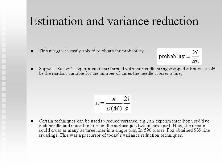
Estimation and variance reduction n This integral is easily solved to obtain the probability n Suppose Buffon’s experiment is performed with the needle being dropped n times. Let M be the random variable for the number of times the needle crosses a line, n Certain techniques can be used to reduce variance, e. g. , an experimenter Fox used five inch needle and made the lines on the surface just two inches apart. Now, the needle could cross as many as three lines in a single toss. In 590 tosses, Fox obtained 939 line crossings. This was a precursor of today’s variance reduction techniques.

Variance Reduction n There are several ways to reduce the variance u Importance Sampling u Stratified Sampling u Quasi-random Sampling u Metropolis Random Mutations

Simulation Often rely on Other Distributions Analytical transformations n Box-Muller Transformation n Rejection method n

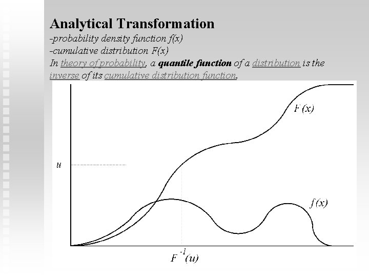
Analytical Transformation -probability density function f(x) -cumulative distribution F(x) In theory of probability, a quantile function of a distribution is the inverse of its cumulative distribution function.

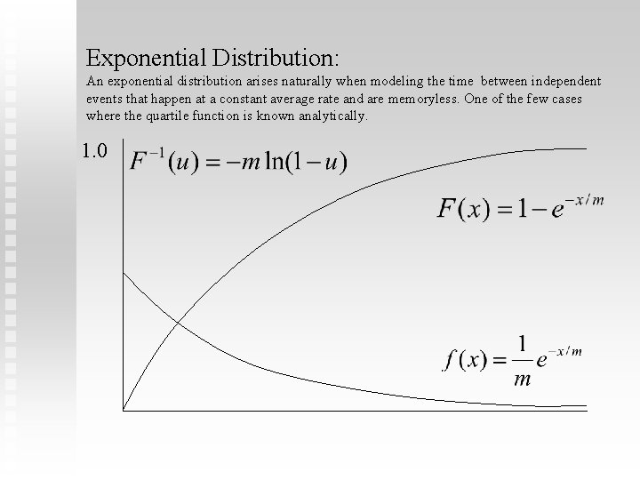
Exponential Distribution: An exponential distribution arises naturally when modeling the time between independent events that happen at a constant average rate and are memoryless. One of the few cases where the quartile function is known analytically. 1. 0

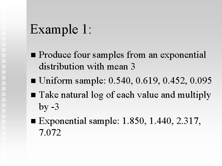
Example 1: Produce four samples from an exponential distribution with mean 3 n Uniform sample: 0. 540, 0. 619, 0. 452, 0. 095 n Take natural log of each value and multiply by -3 n Exponential sample: 1. 850, 1. 440, 2. 317, 7. 072 n

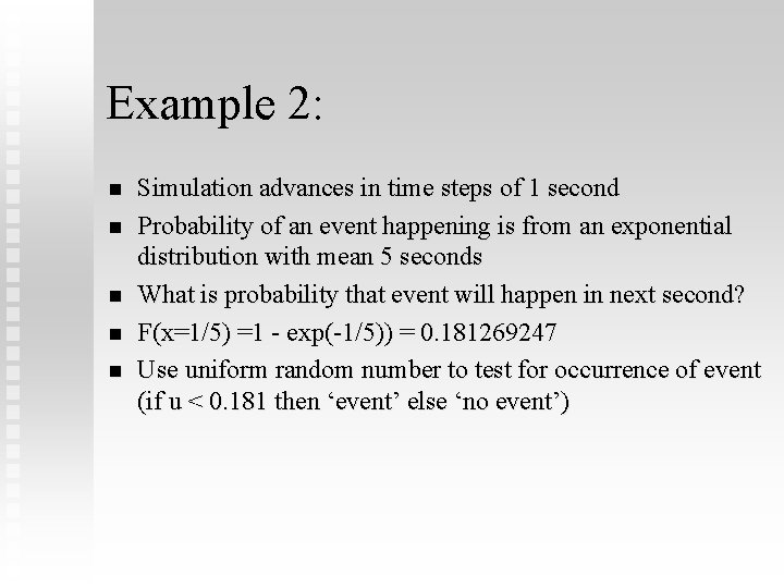
Example 2: n n n Simulation advances in time steps of 1 second Probability of an event happening is from an exponential distribution with mean 5 seconds What is probability that event will happen in next second? F(x=1/5) =1 - exp(-1/5)) = 0. 181269247 Use uniform random number to test for occurrence of event (if u < 0. 181 then ‘event’ else ‘no event’)

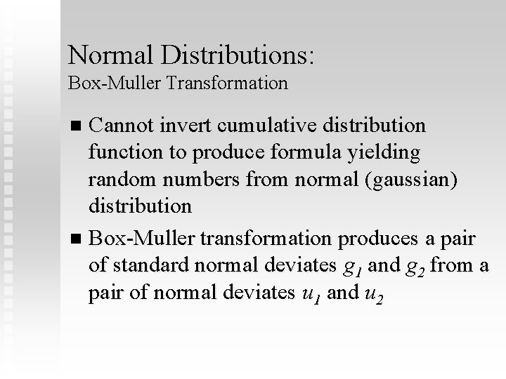
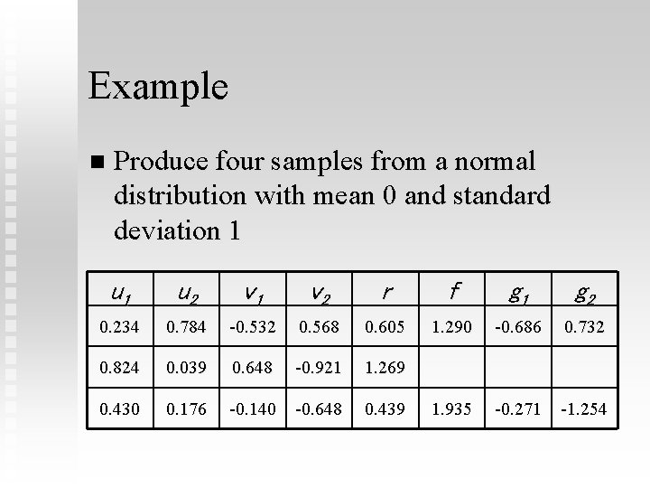
Normal Distributions: Box-Muller Transformation Cannot invert cumulative distribution function to produce formula yielding random numbers from normal (gaussian) distribution n Box-Muller transformation produces a pair of standard normal deviates g 1 and g 2 from a pair of normal deviates u 1 and u 2 n

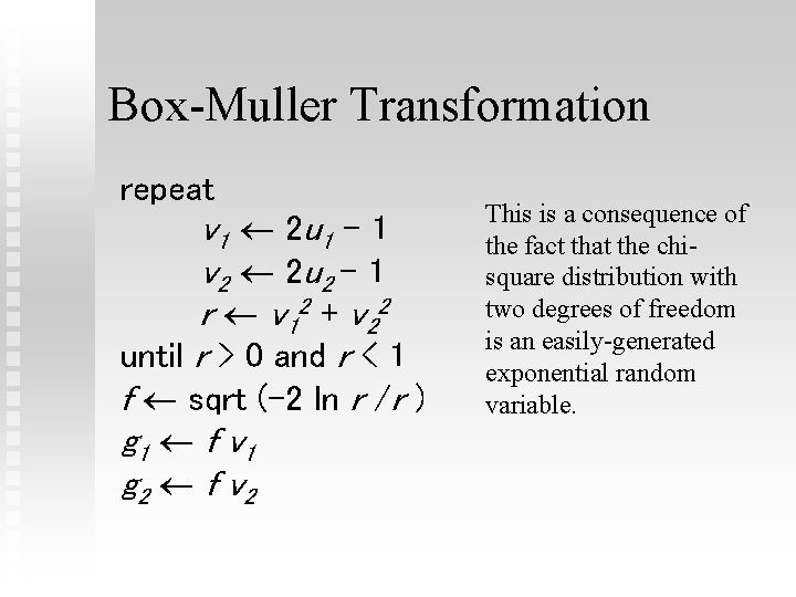
Box-Muller Transformation repeat v 1 2 u 1 - 1 v 2 2 u 2 - 1 r v 12 + v 22 until r > 0 and r < 1 f sqrt (-2 ln r /r ) g 1 f v 1 g 2 f v 2 This is a consequence of the fact that the chisquare distribution with two degrees of freedom is an easily-generated exponential random variable.

Example n Produce four samples from a normal distribution with mean 0 and standard deviation 1 u 2 v 1 v 2 r f g 1 g 2 0. 234 0. 784 -0. 532 0. 568 0. 605 1. 290 -0. 686 0. 732 0. 824 0. 039 0. 648 -0. 921 1. 269 0. 430 0. 176 -0. 140 -0. 648 0. 439 1. 935 -0. 271 -1. 254

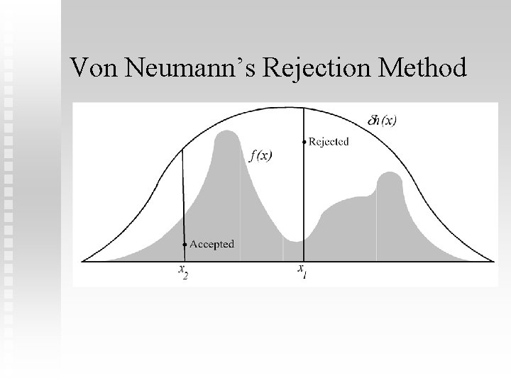
Von Neumann’s Rejection Method

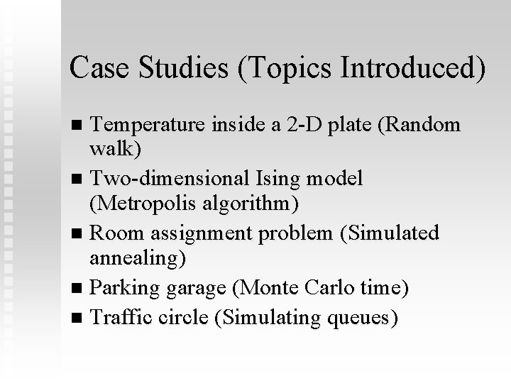
Case Studies (Topics Introduced) Temperature inside a 2 -D plate (Random walk) n Two-dimensional Ising model (Metropolis algorithm) n Room assignment problem (Simulated annealing) n Parking garage (Monte Carlo time) n Traffic circle (Simulating queues) n

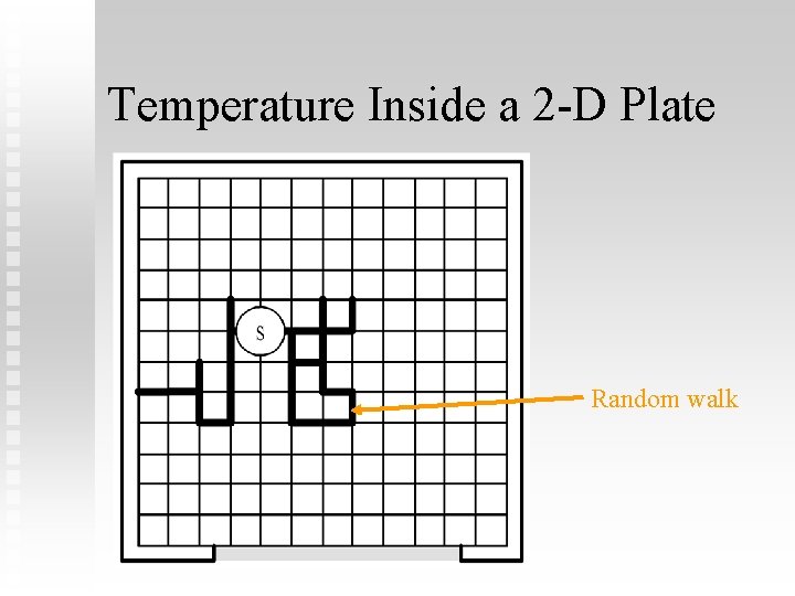
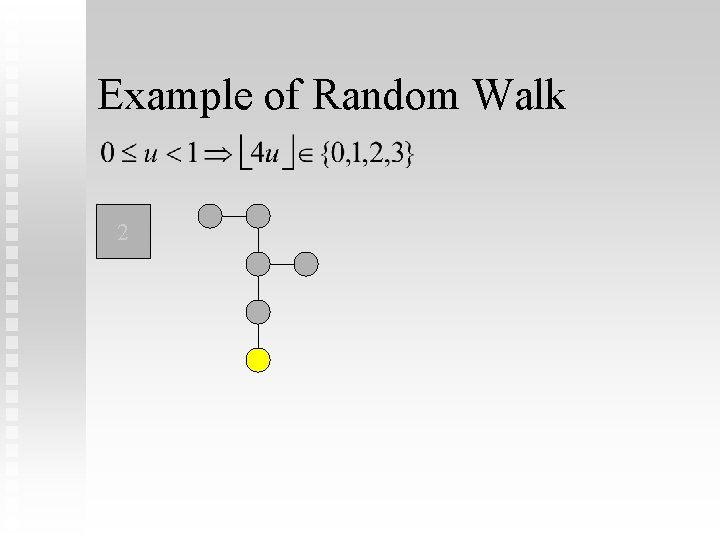
Temperature Inside a 2 -D Plate Random walk

Example of Random Walk 132

Parking Garage Parking garage has S stalls n Car arrivals fit Poisson distribution with mean A: Exponentially distributed interarrival times n Stay in garage fits a normal distribution with mean M and standard deviation M/S n

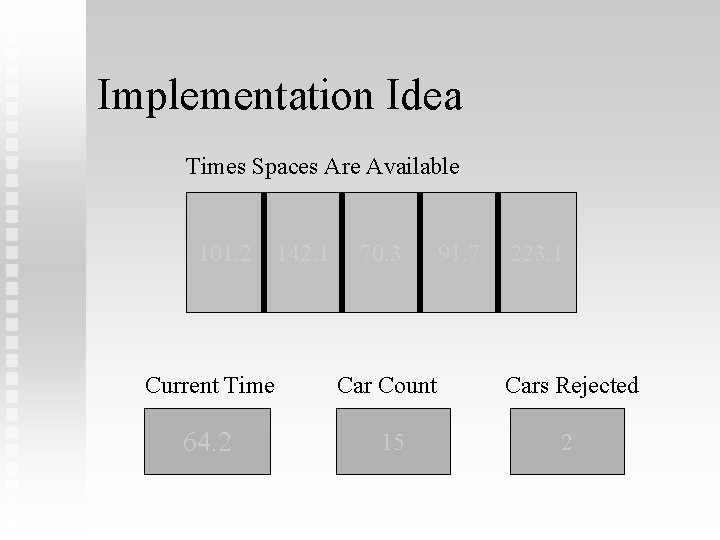
Implementation Idea Times Spaces Are Available 101. 2 142. 1 70. 3 91. 7 223. 1 Current Time Car Count Cars Rejected 64. 2 15 2

Summary n Concepts revealed in case studies u Monte Carlo time u Random walk u Metropolis algorithm u Simulated annealing u Modeling queues