Lecture 10 Joint Random Variables Part 2 IE

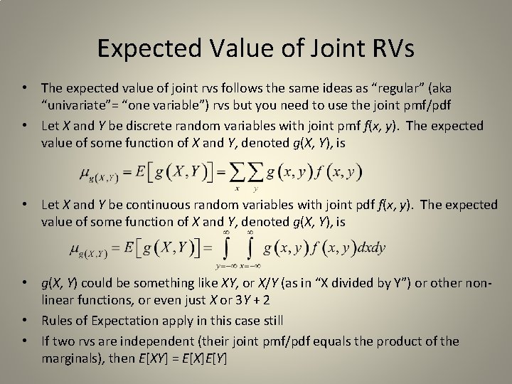
Expected Value of Joint RVs • The expected value of joint rvs follows the same ideas as “regular” (aka “univariate”= “one variable”) rvs but you need to use the joint pmf/pdf • Let X and Y be discrete random variables with joint pmf f(x, y). The expected value of some function of X and Y, denoted g(X, Y), is • Let X and Y be continuous random variables with joint pdf f(x, y). The expected value of some function of X and Y, denoted g(X, Y), is • g(X, Y) could be something like XY, or X/Y (as in “X divided by Y”) or other nonlinear functions, or even just X or 3 Y + 2 • Rules of Expectation apply in this case still • If two rvs are independent (their joint pmf/pdf equals the product of the marginals), then E[XY] = E[X]E[Y]

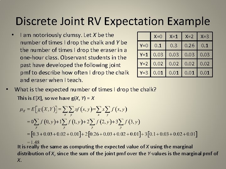
Discrete Joint RV Expectation Example • I am notoriously clumsy. Let X be the X=0 number of times I drop the chalk and Y be Y=0 0. 1 the number of times I drop the eraser in a Y=1 0. 03 one-hour class. Observant students in the Y=2 0. 02 past have developed the following joint Y=3 0. 01 pmf to describe how often I drop the chalk and eraser when I teach. • What is the expected number of times I drop the chalk? X=1 X=2 X=3 0. 26 0. 1 0. 03 0. 02 0. 01 This is E[X], so we have g(X, Y) = X It is really the same as computing the expected value of X using the marginal distribution of X, since the sum of the joint pmf over the Y-values is the marginal pmf of X.

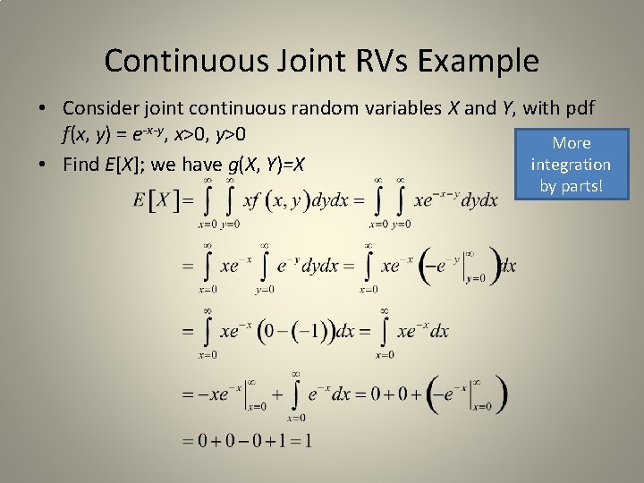
Continuous Joint RVs Example • Consider joint continuous random variables X and Y, with pdf f(x, y) = e-x-y, x>0, y>0 More integration • Find E[X]; we have g(X, Y)=X by parts!

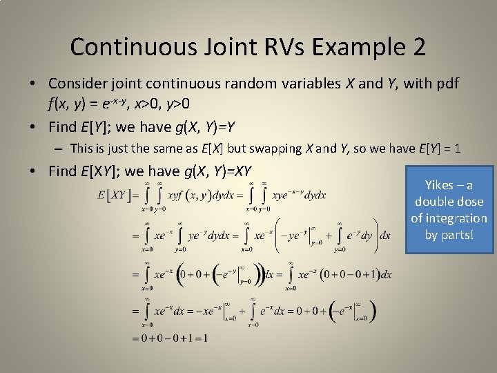
Continuous Joint RVs Example 2 • Consider joint continuous random variables X and Y, with pdf f(x, y) = e-x-y, x>0, y>0 • Find E[Y]; we have g(X, Y)=Y – This is just the same as E[X] but swapping X and Y, so we have E[Y] = 1 • Find E[XY]; we have g(X, Y)=XY Yikes – a double dose of integration by parts!

Covariance • If two rvs are related through a joint pmf/pdf, we may ask: – If one goes up, does the other go down? – Do large changes in one correspond to large changes in the other? • These questions are answered by the covariance, Cov(X, Y) = σXY – – Describes nature of linear relationship between two rvs Same idea for discrete or continuous joint rvs Definition: Cov(X, Y) = σXY = E[(X-μX)(Y-μY)] may be positive or negative!!! Easier computation: Cov(X, Y) = σXY = E[XY] – μXμY • Interpreting the covariance – If two rvs are independent, then Cov(X, Y) = 0 – The reverse is not true. If the covariance between two random variables is zero, we cannot conclude that the two random variables are independent • independence is a result of the pmf/pdf relationship described in the previous lecture – An important factor is the sign of the covariance • Positive indicates an increase in one rv is associated with an increase in the other • Negative indicates a decrease in one rv is associated with an increase in the other

Covariance Example • If E[X] = 1, E[Y] = -1, and E[XY] = 4, what is the covariance of X and Y? Cov(X, Y) = E[XY] – μXμY = E[XY] – E[X] E[Y] = 4 – (1)(-1) = 5 X and Y have positive covariance • If E[W] = 10, E[Z] = -10, and E[WZ] = 400, what is the covariance of W and Z? Cov(W, Z) = E[WZ] – μWμZ = E[WZ] – E[W] E[Z] = 400 – (10)(-10) = 500 W and Z have positive covariance • Are the relationships between X and Y and W and Z very different? – Maybe , maybe not. The covariance is not unitless, so it is not meaningful to compare the covariances of different pairs of rvs

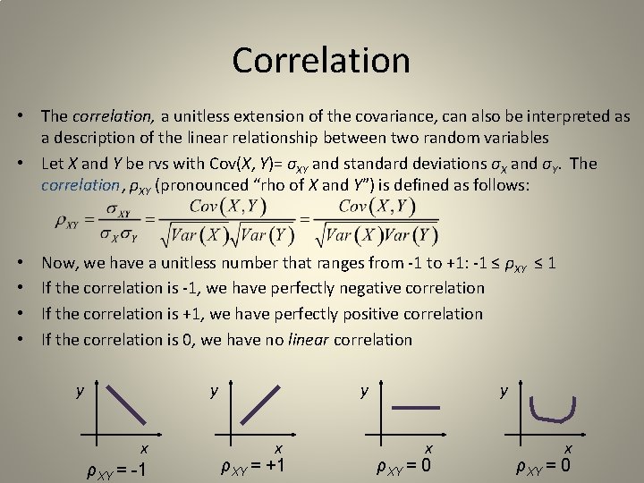
Correlation • The correlation, a unitless extension of the covariance, can also be interpreted as a description of the linear relationship between two random variables • Let X and Y be rvs with Cov(X, Y)= σXY and standard deviations σX and σY. The correlation, ρXY (pronounced “rho of X and Y”) is defined as follows: • • Now, we have a unitless number that ranges from -1 to +1: -1 ≤ ρXY ≤ 1 If the correlation is -1, we have perfectly negative correlation If the correlation is +1, we have perfectly positive correlation If the correlation is 0, we have no linear correlation y y x ρXY = -1 y x ρXY = +1 y x ρXY = 0

Correlation Example • Assume E[X] = ½ , E[Y] = 1/3, E[XY] = ¼, Var[X] = ¼ and Var[Y] = 1/12 • What is the correlation of X and Y? • First, compute the covariance Cov(X, Y) = E[XY] – μXμY = E[XY] – E[X] E[Y] = ¼ - ½(1/3) = 1/12 • Now, compute the correlation • X and Y are somewhat positively correlated

Related reading • Montgomery and Runger, section 5 -2 – The captions of Figures 5 -14, 5 -15, and 5 -16 should refer to Examples 5 -21, 5 -22, and 5 -23, respectively. • Some links that might help (maybe) – Nice pictures of correlations are at http: //en. wikipedia. org/wiki/Correlation – http: //cnx. org/content/m 11248/latest/ • Now you are ready to do HW 10