Lecture 10 Correlation and Regression Introduction to Correlation

Lecture 10 Correlation and Regression

Introduction to Correlation n We’ve been studying the differences between groups… n Now, let’s describe the relationship between variables n Two “interwoven” areas of statistics concern the relationship between variables: correlation and regression

n Correlations describe the relationship between two variables – They refer to the extent to which one variable is related to another variable – The variables that are observed typically occur naturally. Usually there is no manipulation n Correlations exist when: – a change in one variable is accompanied by a consistent change in the other – Requires 2 scores for each individual (usually identified by X and Y) For example, when you applied to college you probably had to submit your SAT scores. Admissions counselors often look at SAT scores because there is a relationship between SAT scores and collegiate achievement. Such that people who did poorly on the SATs tend to get poor grades in college and people that did well on the SATs get good grades in college.

Notation n Correlations are symbolized as r, when referring to correlations based on samples – Correlations are almost always based on samples n (rho) is the symbol when referring to a correlation that is presumed to exist (or not; if a null hypothesis) in a population

Characteristics of Correlation n Direction n Form n Degree

Direction of the Relationship n There are three directions for correlations: – Positive correlation: this is when an increase in one variable is accompanied by an increase in the other. Variables go in the same direction: low score on one low score on the other, hi score on one hi on the other. (sign is +) – Negative correlation: this is when an increase in one variable is accompanied by a decrease in the other. Variables go in opposite directions: low score on one hi score on the other. (sign is -) – Zero correlation: this is when there is no relationship between the two variables

Scatterplots n Scatterplots are graphic representations that display correlations - allow you to see general patterns or trends n In scatterplots the X values are placed on the horizontal axis and the Y values are placed on the vertical axis n Each individual is plotted as a single data point

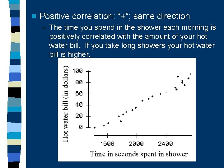
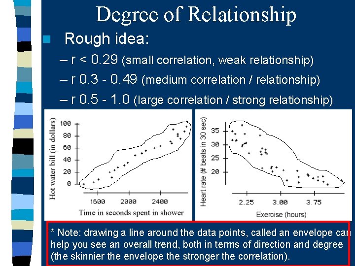
n Positive correlation: “+”; same direction – The time you spend in the shower each morning is positively correlated with the amount of your hot water bill. If you take long showers your hot water bill is higher.

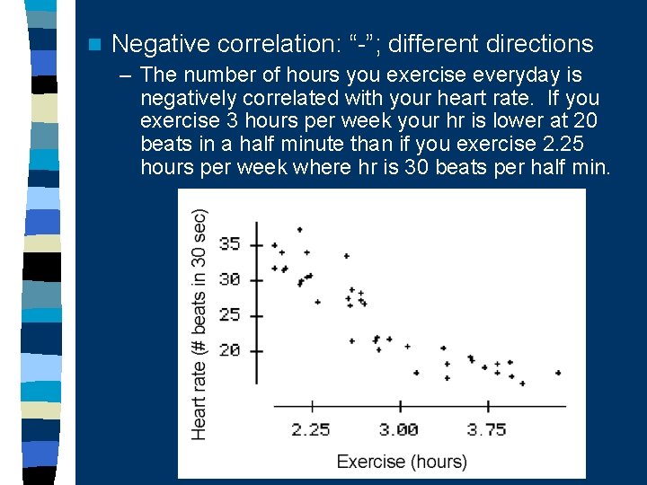
n Negative correlation: “-”; different directions – The number of hours you exercise everyday is negatively correlated with your heart rate. If you exercise 3 hours per week your hr is lower at 20 beats in a half minute than if you exercise 2. 25 hours per week where hr is 30 beats per half min.

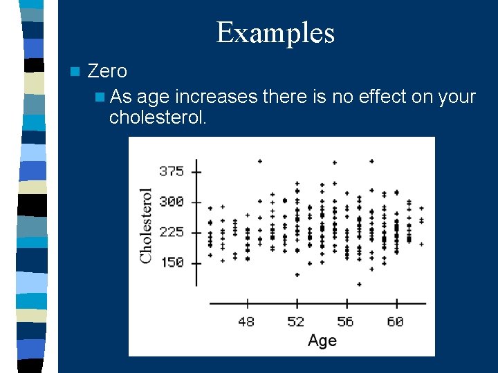
Examples n Zero n As age increases there is no effect on your cholesterol.

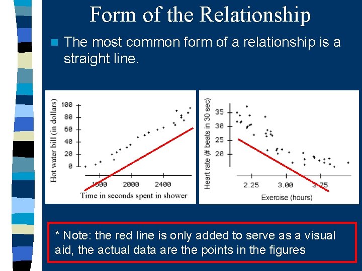
Form of the Relationship n The most common form of a relationship is a straight line. * Note: the red line is only added to serve as a visual aid, the actual data are the points in the figures

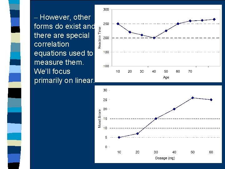
– However, other forms do exist and there are special correlation equations used to measure them. We’ll focus primarily on linear.

Degree of the Relationship n A correlation measures how well the data fit the specific form being considered. – Remember the most common form is going to be linear, so the degree will measure how well the data points fit a straight line. A perfect correlation is identified by a 1. 0 or 1. 0 and indicates a perfect fit. A correlation of 0 indicates no fit at all. Intermediate values are going to represent the degree to which there is a consistent, predictable relationship in the data. (Nothing greater than 1 or -1). n Remember look at degree and direction separately (you can have a perfect neg. correlation). n

Degree of Relationship n Rough idea: – r < 0. 29 (small correlation, weak relationship) – r 0. 3 - 0. 49 (medium correlation / relationship) – r 0. 5 - 1. 0 (large correlation / strong relationship) * Note: drawing a line around the data points, called an envelope can help you see an overall trend, both in terms of direction and degree (the skinnier the envelope the stronger the correlation).

Why are Correlations Used? (1) Prediction: If 2 variables are known to be related in a systematic way we can use one variable to predict the other. – Admissions counselors want to see the SATs of applicants to their college because they use it to predict how well that student might do if they are admitted. Hi SATs predict Hi grades. Prediction is not perfectly accurate, but helpful (2) Validity: Remember validity is the likelihood that the test we are using measure what we want it to measure. – Say we come up with a new measure to test for depression. If our measure truly measures depression it should correlate with other measures of depression.

Why are Correlations Used? (3) Reliability: Remember reliability is the likelihood that our measurement is stable. – If I measure your weight on Tues. it should be very similar on Wed. and Thurs. If not we would suspect that something is wrong with our scale. When reliability is high the correlation between on weight on Tues. should be highly correlated with our weight on Wed. and Thurs. (4) Theory Verification: many scientific theories make specific predictions about the relationship between variables – If I have a theory that the oldest child in the family makes earns the highest salary. Then I should expect that there is a correlation between birth order and salary, such that younger children earn less and oldest children earn more.

Putting it Together n If the world were fair, would you expect a positive or negative relationship between number of hours worked each week and salary? n Data suggest that on average children from large families have lower IQs than children from small families. Do these data suggest a positive or negative correlation between family size and average IQ?

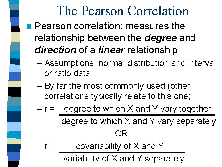
The Pearson Correlation n Pearson correlation: measures the relationship between the degree and direction of a linear relationship. – Assumptions: normal distribution and interval or ratio data – By far the most commonly used (other correlations typically relate to this one) – r = degree to which X and Y vary together degree to which X and Y vary separately OR –r= covariability of X and Y separately

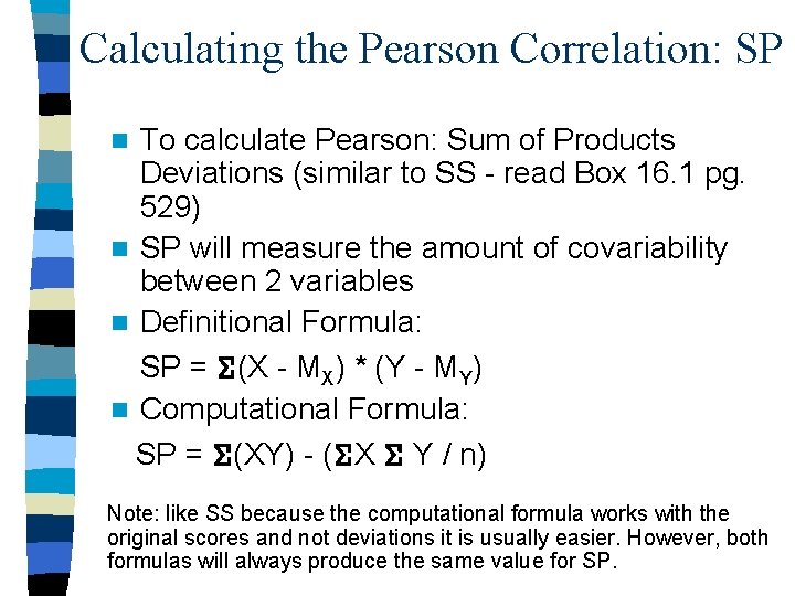
Calculating the Pearson Correlation: SP To calculate Pearson: Sum of Products Deviations (similar to SS - read Box 16. 1 pg. 529) n SP will measure the amount of covariability between 2 variables n Definitional Formula: SP = (X - MX) * (Y - MY) n Computational Formula: SP = (XY) - ( X Y / n) n Note: like SS because the computational formula works with the original scores and not deviations it is usually easier. However, both formulas will always produce the same value for SP.

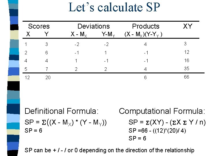
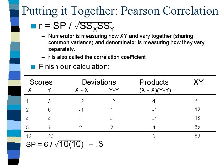
Let’s calculate SP Scores X Y Deviations X - MX Y-MY Products XY (X - MX)(Y-YY ) 1 3 -2 -2 4 3 2 6 -1 12 4 4 1 -1 -1 16 5 7 2 2 4 35 12 20 6 66 Definitional Formula: SP = ((X - MX) * (Y - MY)) SP = 6 Computational Formula: SP = (XY) - ( X Y / n) SP =66 - ((12)*(20)/ 4) SP = 6 SP can be + / - / or 0 depending on the direction of the relationship

Putting it Together: Pearson Correlation nr = SP / SSXSSY – Numerator is measuring how XY and vary together (sharing common variance) and denominator is measuring how they vary separately. – r is also called the correlation coefficient n Finish our calculation: Scores X Deviations Products XY Y X-X Y-Y (X - X)(Y-Y) 1 3 -2 -2 4 3 2 6 -1 12 4 4 1 -1 -1 16 5 7 2 2 4 35 12 20 6 66 SP = 6 / 10(10) =. 6

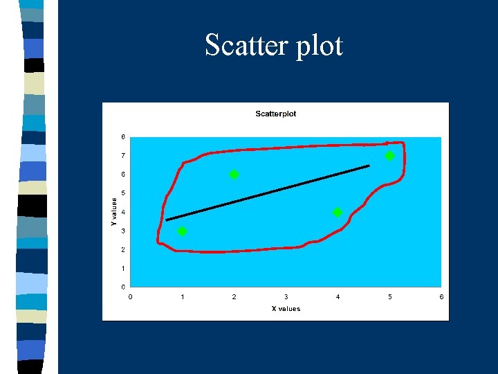
Scatter plot

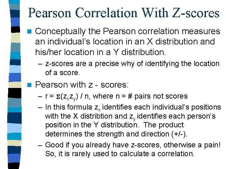
Pearson Correlation With Z-scores n Conceptually the Pearson correlation measures an individual’s location in an X distribution and his/her location in a Y distribution. – z-scores are a precise why of identifying the location of a score. n Pearson with z - scores: – r = (zxzy) / n, where n = # pairs not scores – In this formula zx identifies each individual’s positions with the X distribtion and zy identifies each person’s position in the Y distribution. The product determines the strength and direction (+/-). – Good if you already have z-scores, otherwise a pain! So, it is rarely used to calculate a correlation.

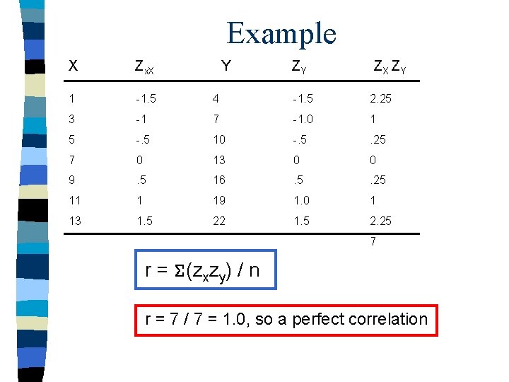
Example X Zx. X Y ZY Z X ZY 1 -1. 5 4 -1. 5 2. 25 3 -1 7 -1. 0 1 5 -. 5 10 -. 5 . 25 7 0 13 0 0 9 . 5 16 . 5 . 25 11 1 19 1. 0 1 13 1. 5 22 1. 5 2. 25 7 r = (zxzy) / n r = 7 / 7 = 1. 0, so a perfect correlation

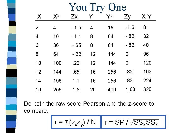
You Try One X X 2 Zx Y Y 2 Zy XY 2 4 -1. 5 4 16 -1. 6 8 4 16 -1. 1 8 64 -. 82 32 6 36 -. 65 8 64 -. 82 48 8 64 -. 22 12 144 0 96 10 100 . 22 12 144 0 12 144 . 65 16 256 . 82 192 14 196 1. 1 16 256 . 82 224 16 256 1. 5 20 400 1. 63 320 Do both the raw score Pearson and the z-score to compare. r = (zxzy) / N r = SP / SSXSSY

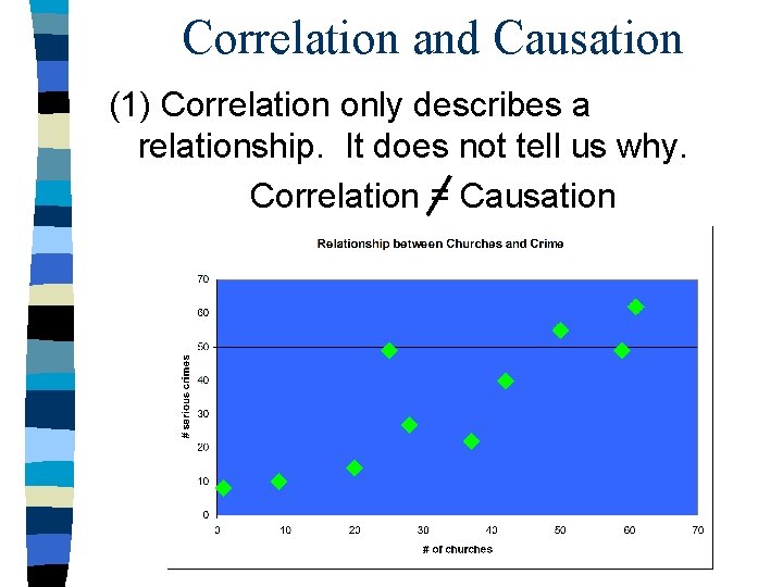
Correlation and Causation (1) Correlation only describes a relationship. It does not tell us why. Correlation = Causation

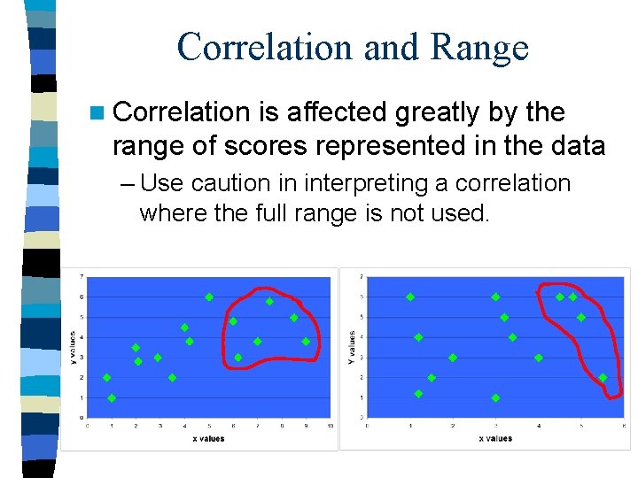
Correlation and Range n Correlation is affected greatly by the range of scores represented in the data – Use caution in interpreting a correlation where the full range is not used.

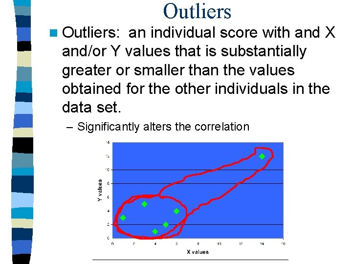
Outliers n Outliers: an individual score with and X and/or Y values that is substantially greater or smaller than the values obtained for the other individuals in the data set. – Significantly alters the correlation

Interpreting the Strength of the Relationship We already know the degree of the relationship between 2 variables can be between -1. 0 and 1. 0 n How do we measure the strength of a correlation? n – r 2 = measures the proportion of the variability in the data that is explained by the relationship between X and Y. – Coefficient of determination - because it measure the proportion of variability in 1 variable that can be determined from the relationship with the other. • e. g. r =. 80 then r 2 =. 64 or 64% of the variability in X can be explained by Y. • OR r =. 60 then r 2 =. 36 or 36% of the variability in X can be explained by Y. • Finally when r = 1. 0 then r 2 = 1. 0 or 100% of the variability in X can be explained by Y.

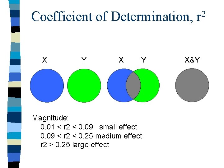
Coefficient of Determination, r 2 X Y Magnitude: 0. 01 < r 2 < 0. 09 small effect 0. 09 < r 2 < 0. 25 medium effect r 2 > 0. 25 large effect X&Y

Regression Toward the Mean n Regression toward the mean is a simple observation about correlations. – When there is a less than perfect correlation between two variables, extreme scores (hi or lo) on one variable tend to be paired with less extreme scores on the second variable • E. g. If we are correlated the intelligence of fathers and their children. It is likely that if the father has an extremely low IQ the child’s IQ will be fairly close to the population mean IQ. If the child has an extremely high IQ it is likely that the father’s will be lower, closer to the mean. (However, there may be exceptions to this).

Hypothesis Tests with Pearson (1) State the Hypothesis (Remember we want to know if the correlation exists in the population or is due to chance) * H 0 = = 0 or H 0 = 0 or 0 * H 1 = = 0 or H 1 = > 0 or < 0 (2) Set critical region in Table B. 6 (must meet or exceed the critical values) need sample size (n) n magnitude of the correlation (independent of sign) n df n – df for Pearson is n-2, where n is sample size. • This is because we have 2 restrictions on variability the mean and also the relationship between X and Y • Or conceptually you have to have 2 points to make a line * Is the correlation from our example problem significant?

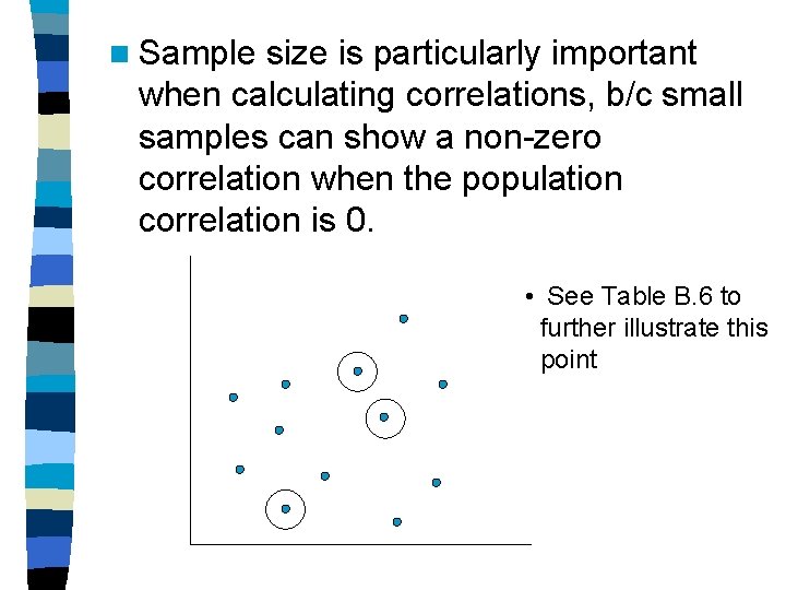
n Sample size is particularly important when calculating correlations, b/c small samples can show a non-zero correlation when the population correlation is 0. • See Table B. 6 to further illustrate this point

In the Literature n. A correlation for the data revealed that amount of education and annual income were significantly related, r = +. 65, n = 30, p <. 01, two-tailed. n With correlation it is useful to report: – The sample size – Calculated value for the correlation – Whether it is significant – The probability – Type of test (1 - or 2 -tailed)

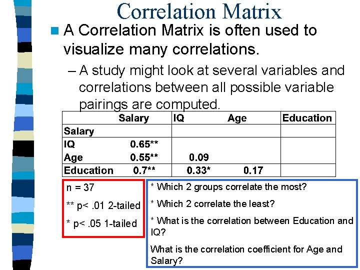
n. A Correlation Matrix is often used to visualize many correlations. – A study might look at several variables and correlations between all possible variable pairings are computed. n = 37 * Which 2 groups correlate the most? ** p<. 01 2 -tailed * Which 2 correlate the least? * p<. 05 1 -tailed * What is the correlation between Education and IQ? What is the correlation coefficient for Age and Salary?

The Spearman Correlation n Uses: (1) Measures the relationship between variables measured on an ordinal scale of measurement. A Pearson with ordinal data. • Remember ordinal scales involved data that are placed into rank order – e. g. It might be easy for an coach to rank order players by their athletic ability, but very difficult to measure athletic ability on some other scale (2) Instead of measuring a linear relationship can measure consistency in a relationship, independent of form NOTE: We’ve been using mostly parametric tests in this class. Parametric tests use actual #s. Non-parametric tests look at ranks only.

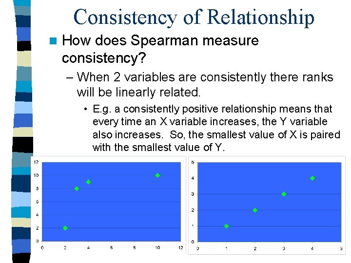
Consistency of Relationship n How does Spearman measure consistency? – When 2 variables are consistently there ranks will be linearly related. • E. g. a consistently positive relationship means that every time an X variable increases, the Y variable also increases. So, the smallest value of X is paired with the smallest value of Y.

How to Use the Spearman: Wanting to Measure Consistency n If the original data are ordinal we can plug them into our formula (Yes, the same formula we used for the Pearson). n If we want to measure consistency independent of form and our original data are not ordinal: – Convert the scores to rank * Note: When there is a consistently one directional relationship between two variables is it said to be monotonic. The Spearman measure the degree to which there is a monotonic relationship between 2 variables.

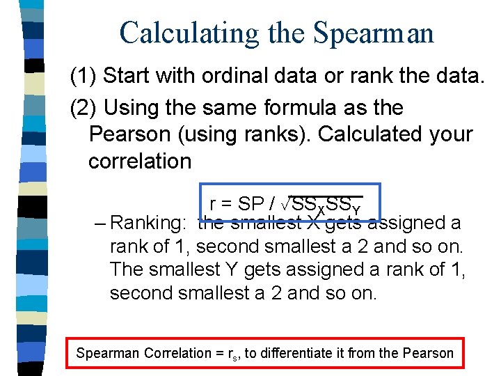
Calculating the Spearman (1) Start with ordinal data or rank the data. (2) Using the same formula as the Pearson (using ranks). Calculated your correlation r = SP / SSXSSY – Ranking: the smallest X gets assigned a rank of 1, second smallest a 2 and so on. The smallest Y gets assigned a rank of 1, second smallest a 2 and so on. Spearman Correlation = rs, to differentiate it from the Pearson

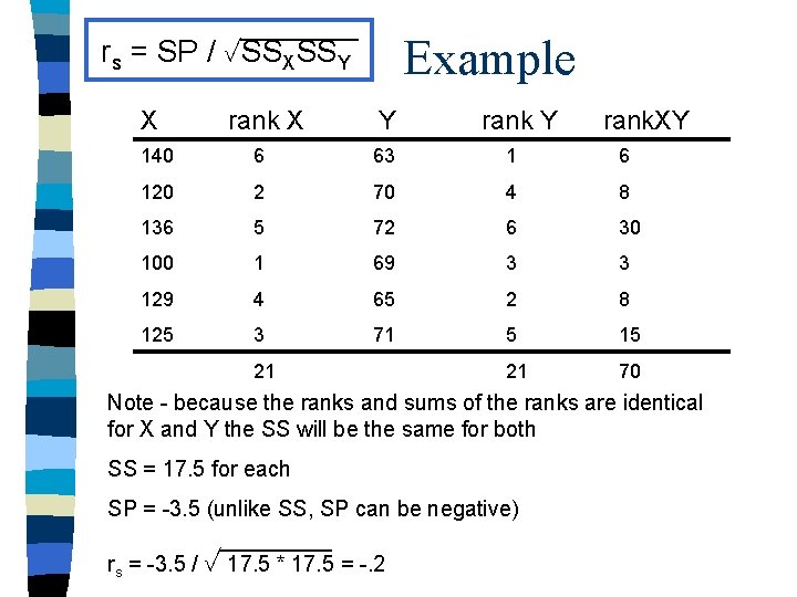
Example rs = SP / SSXSSY X rank X Y rank. XY 140 6 63 1 6 120 2 70 4 8 136 5 72 6 30 100 1 69 3 3 129 4 65 2 8 125 3 71 5 15 21 70 21 Note - because the ranks and sums of the ranks are identical for X and Y the SS will be the same for both SS = 17. 5 for each SP = -3. 5 (unlike SS, SP can be negative) rs = -3. 5 / 17. 5 * 17. 5 = -. 2

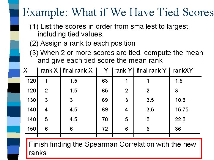
Example: What if We Have Tied Scores (1) List the scores in order from smallest to largest, including tied values. (2) Assign a rank to each position (3) When 2 or more scores are tied, compute the mean and give each tied score the mean rank X final rank X Y rank Y final rank Y rank. XY 120 1 1. 5 63 1 1 1. 5 120 2 1. 5 65 2 2 3 130 3 3 69 3 3. 5 10. 5 140 4 4. 5 69 4 3. 5 15. 75 140 5 4. 5 70 5 5 22. 5 150 6 6 72 6 6 36 Finish finding the Spearman Correlation with the new ranks.

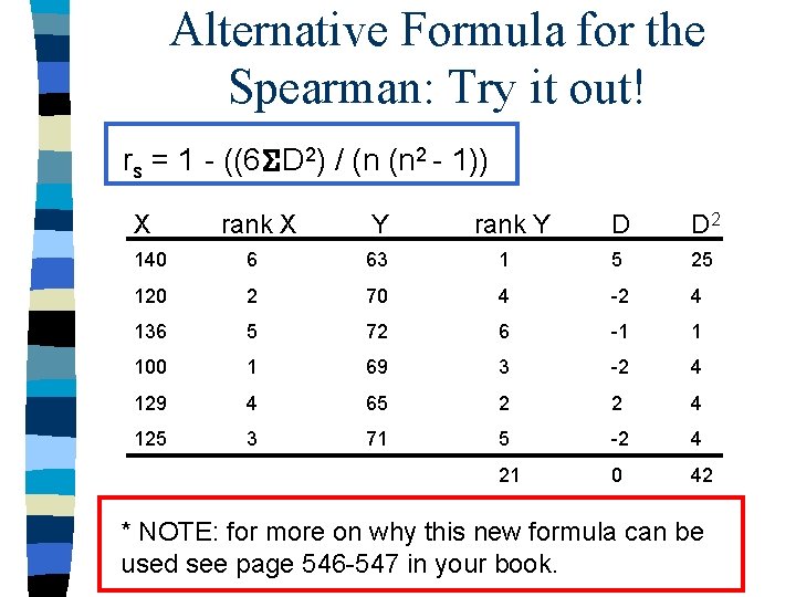
Alternative Formula for the Spearman: Try it out! rs = 1 - ((6 D 2) / (n (n 2 - 1)) X rank X Y rank Y D D 2 140 6 63 1 5 25 120 2 70 4 -2 4 136 5 72 6 -1 1 100 1 69 3 -2 4 129 4 65 2 2 4 125 3 71 5 -2 4 21 0 42 * NOTE: for more on why this new formula can be used see page 546 -547 in your book.

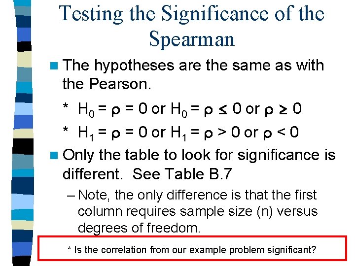
Testing the Significance of the Spearman n The hypotheses are the same as with the Pearson. * H 0 = = 0 or H 0 = 0 or 0 * H 1 = = 0 or H 1 = > 0 or < 0 n Only the table to look for significance is different. See Table B. 7 – Note, the only difference is that the first column requires sample size (n) versus degrees of freedom. * Is the correlation from our example problem significant?

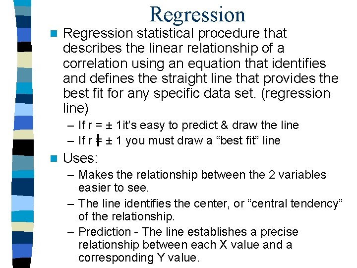
Regression n Regression statistical procedure that describes the linear relationship of a correlation using an equation that identifies and defines the straight line that provides the best fit for any specific data set. (regression line) – If r = ± 1 it’s easy to predict & draw the line – If r = ± 1 you must draw a “best fit” line n Uses: – Makes the relationship between the 2 variables easier to see. – The line identifies the center, or “central tendency” of the relationship. – Prediction - The line establishes a precise relationship between each X value and a corresponding Y value.

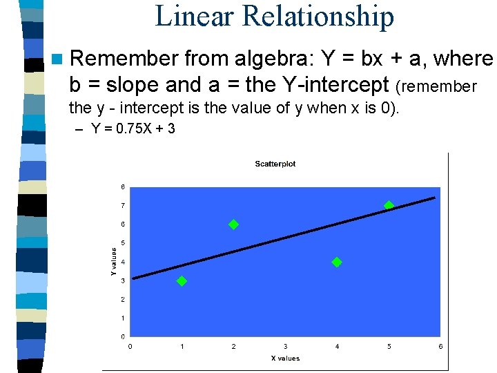
Linear Relationship n Remember from algebra: Y = bx + a, where b = slope and a = the Y-intercept (remember the y - intercept is the value of y when x is 0). – Y = 0. 75 X + 3

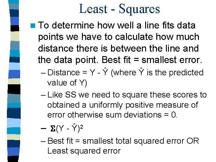
Least - Squares n To determine how well a line fits data points we have to calculate how much distance there is between the line and the data point. Best fit = smallest error. – Distance = Y - Ŷ (where Ŷ is the predicted value of Y) – Like SS we need to square these scores to obtained a uniformly positive measure of error otherwise sum deviations = 0. – (Y - Ŷ)2 – Best fit = smallest total squared error OR Least squared error

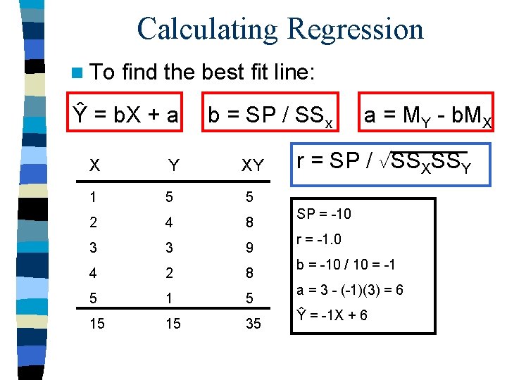
Calculating Regression n To find the best fit line: Ŷ = b. X + a b = SP / SSx X Y XY 1 5 5 2 4 8 3 3 9 4 2 8 5 15 15 35 a = MY - b. MX r = SP / SSXSSY SP = -10 r = -1. 0 b = -10 / 10 = -1 a = 3 - (-1)(3) = 6 Ŷ = -1 X + 6

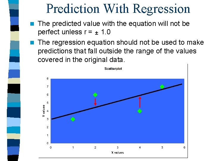
Prediction With Regression The predicted value with the equation will not be perfect unless r = 1. 0 n The regression equation should not be used to make predictions that fall outside the range of the values covered in the original data. n

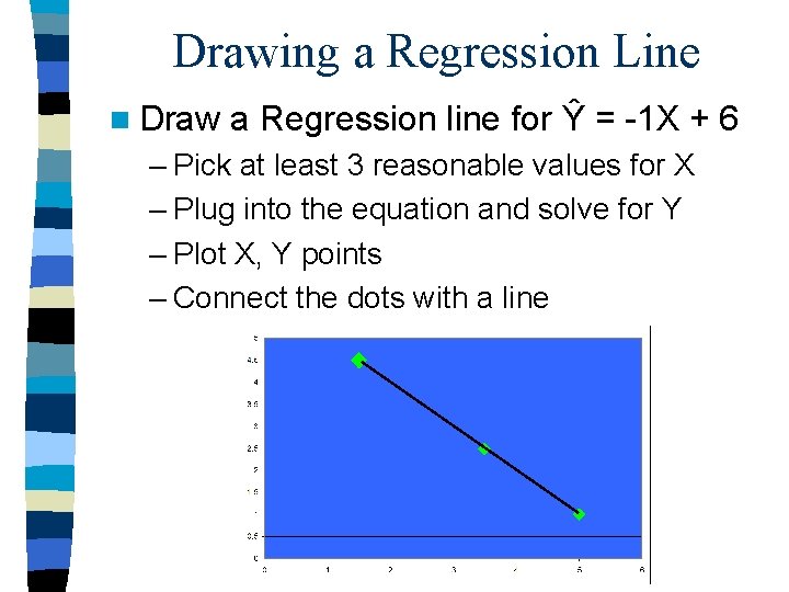
Drawing a Regression Line n Draw a Regression line for Ŷ = -1 X + 6 – Pick at least 3 reasonable values for X – Plug into the equation and solve for Y – Plot X, Y points – Connect the dots with a line

Standard Error of the Estimate n Accuracy depends on how well the line fits the points (it’s possible to have the same regression line for 2 different data sets and where one has very little error and the other a lot, see page 550 in the book) n Standard error of estimate give the measure of the standard distance between a regression line and the actual data points – SSerror = (Y - Ŷ)2 – Variance = SS / df – Standard error of estimate = variance

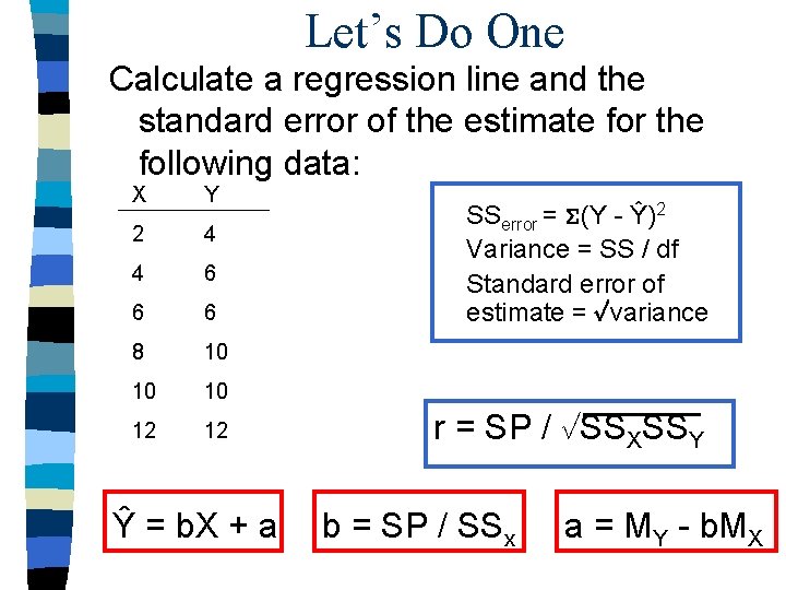
Let’s Do One Calculate a regression line and the standard error of the estimate for the following data: X Y 2 4 4 6 6 6 8 10 10 10 12 12 Ŷ = b. X + a SSerror = (Y - Ŷ)2 Variance = SS / df Standard error of estimate = variance r = SP / SSXSSY b = SP / SSx a = MY - b. MX

Homework: Chapter 16 n 1, 2, 5, 6, 8, 11, 12, 13, 15, 18, 25, 26, 27