Lecture 10 A Matrix Algebra Matrices An array

Lecture 10 A: Matrix Algebra

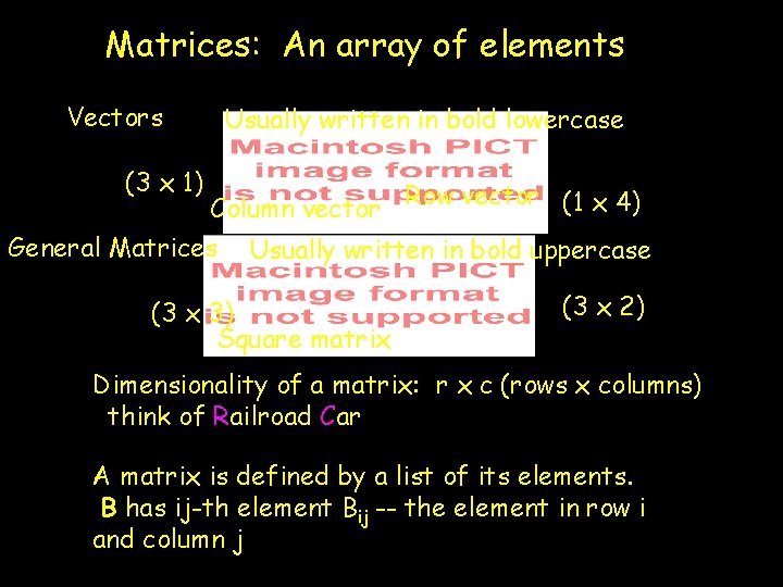
Matrices: An array of elements Vectors Usually written in bold lowercase (3 x 1) Column vector Row vector (1 x 4) General Matrices Usually written in bold uppercase (3 x 3) Square matrix (3 x 2) Dimensionality of a matrix: r x c (rows x columns) think of Railroad Car A matrix is defined by a list of its elements. B has ij-th element Bij -- the element in row i and column j

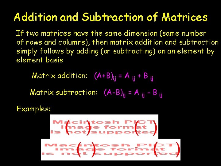
Addition and Subtraction of Matrices If two matrices have the same dimension (same number of rows and columns), then matrix addition and subtraction simply follows by adding (or subtracting) on an element by element basis Matrix addition: (A+B)ij = A ij +B Matrix subtraction: (A-B)ij = A ij ij -B ij Examples: ( ) ( ) (- )

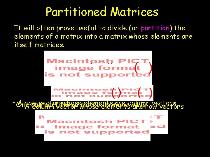
Partitioned Matrices It will often prove useful to divide (or partition) the elements of a matrix into a matrix whose elements are itself matrices. … … … () ( ) • One A row vector whose elements are column vectors partition a whose matrix in many ways A can column vector elements are row vectors

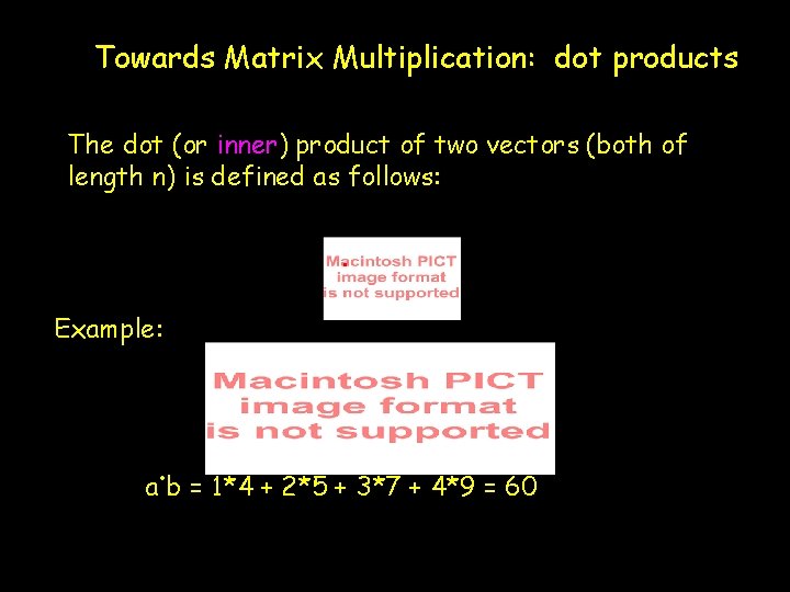
Towards Matrix Multiplication: dot products The dot (or inner) product of two vectors (both of length n) is defined as follows: . Example: . a b = 1*4 + 2*5 + 3*7 + 4*9 = 60

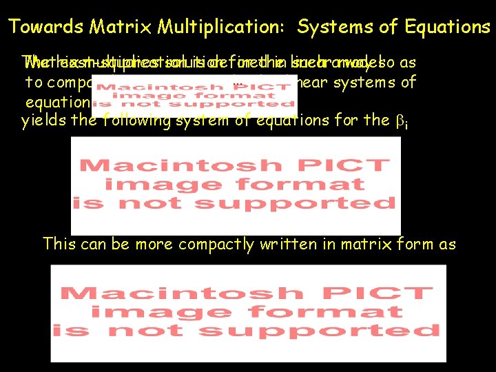
Towards Matrix Multiplication: Systems of Equations The least-squares solution for the Matrix multiplication is defined in linear such amodel way so as to compactly represent and…solve linear systems of equations. yields the following system of equations for the bi This can be more compactly written in matrix form as

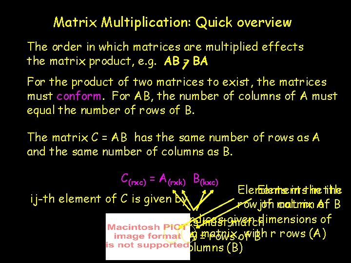
Matrix Multiplication: Quick overview The order in which matrices are multiplied effects the matrix product, e. g. AB = BA For the product of two matrices to exist, the matrices must conform. For AB, the number of columns of A must equal the number of rows of B. The matrix C = AB has the same number of rows as A and the same number of columns as B. C(rxc) = A(rxk) B(kxc) Elements in the ith ij-th element of C is given by column A of B rowjth of matrix Outer indices dimensions of Inner indices mustgiven match resulting with columns of A =matrix, rows of B r rows (A) and c columns (B)

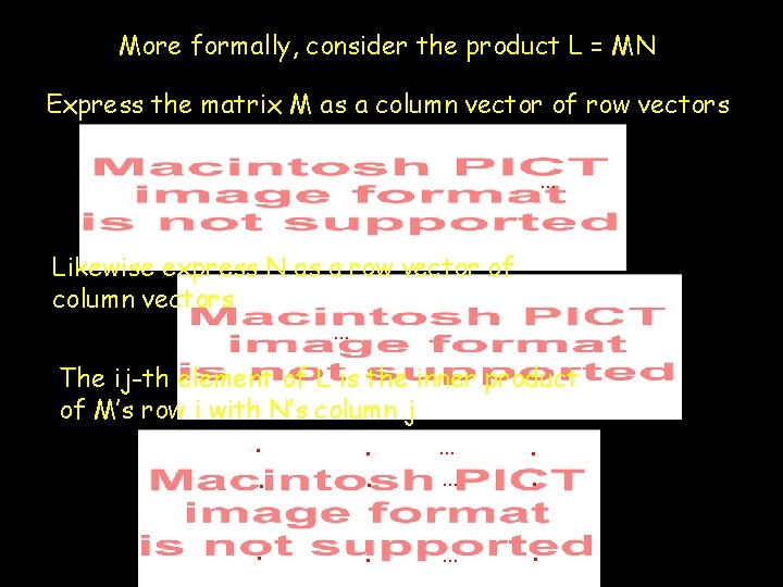
More formally, consider the product L = MN Express the matrix M as a column vector of row vectors … Likewise express N as a row vector of column vectors … The ij-th element of L is the inner product of M’s row i with N’s column j. …. . . … .

Examples ( )( ) ( ( ) )

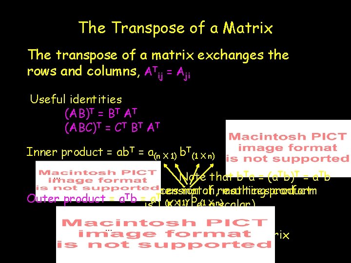
The Transpose of a Matrix The transpose of a matrix exchanges the rows and columns, ATij = Aji Useful identities (AB)T = BT AT (ABC)T = CT BT AT Inner product = ab. T = a(n X 1) b. T(1 X n) … Note that b. Ta = (a. Tb)T = a. Tb Indices Dimension match, of resulting matricesproduct conform T T Outer product = a b =isa 1 (n b (1 Xa n)scalar) XX 11)(i. e. … Resulting product is an nxn matrix

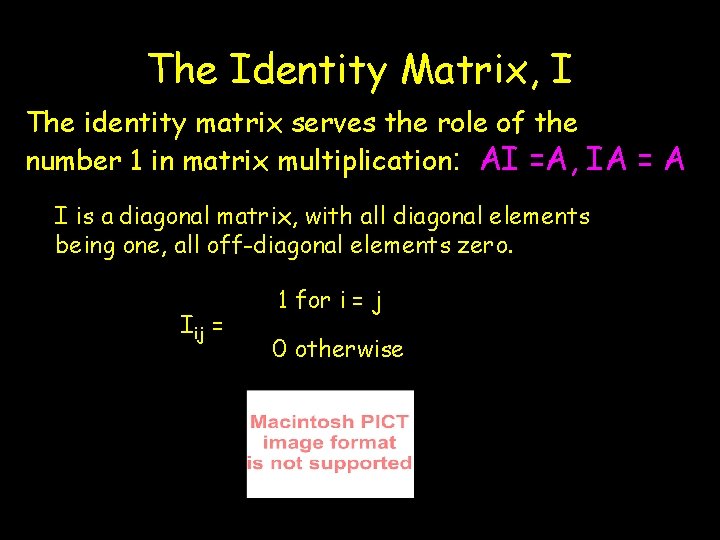
The Identity Matrix, I The identity matrix serves the role of the number 1 in matrix multiplication: AI =A, IA = A I is a diagonal matrix, with all diagonal elements being one, all off-diagonal elements zero. Iij = 1 for i = j 0 otherwise

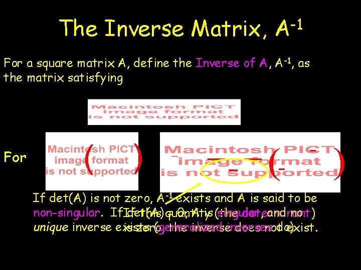
The Inverse Matrix, -1 A For a square matrix A, define the Inverse of A, A-1, as the matrix satisfying For ( ) ( If det(A) is not zero, A-1 exists and A is said to be non-singular. If det(A) = 0, A is (the singular, and no this quantity determinant) unique inverse exists (generalized do) is zero, the inverses does not exist. )

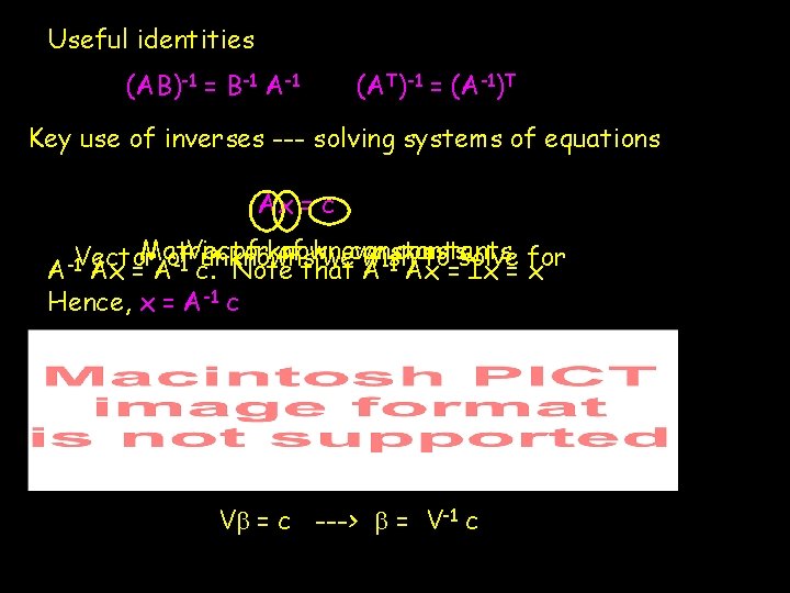
Useful identities (AB)-1 = B-1 A-1 (AT)-1 = (A-1)T Key use of inverses --- solving systems of equations Ax = c Matrix Vector of known constants wish to=solve -1 A Ax Ix = for x Hence, x = A-1 c unknowns we -1 c. A-1 Vector Ax = Aof Note that Vb = c ---> b = V-1 c

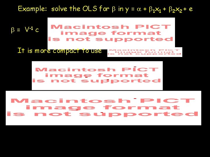
Example: solve the OLS for b in y = a + b 1 x 1 + b 2 x 2 + e b = V-1 c It is more compact to use - - -

- ( - ) If r 12 = 0, these reduce to the two univariate slopes,

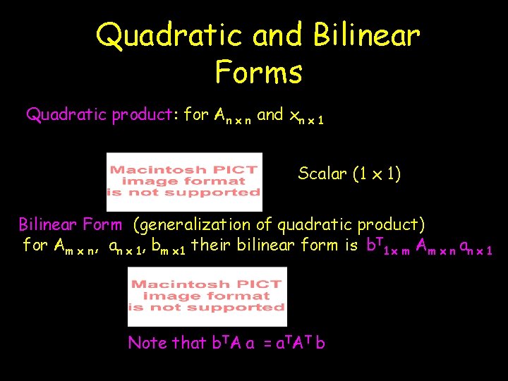
Quadratic and Bilinear Forms Quadratic product: for An x n and xn x 1 Scalar (1 x 1) Bilinear Form (generalization of quadratic product) for Am x n, an x 1, bm x 1 their bilinear form is b. T 1 x m Am x n an x 1 Note that b. TA a = a. TAT b

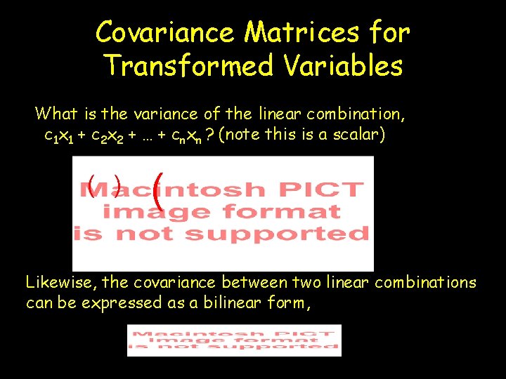
Covariance Matrices for Transformed Variables What is the variance of the linear combination, c 1 x 1 + c 2 x 2 + … + cnxn ? (note this is a scalar) ( Likewise, the covariance between two linear combinations can be expressed as a bilinear form,

Now suppose we transform one vector of random variables into another vector of random variables Transform x into (i) yk x 1 = Ak x n xn x 1 (ii) zm x 1 = Bm x n xn x 1 The covariance between the elements of these two transformed vectors of the origin is a k x m covariance matrix = AVBT For example, the covariance between yi and yj is given by the ij-th element of AVAT Likewise, the covariance between yi and zj is given by the ij-th element of AVBT

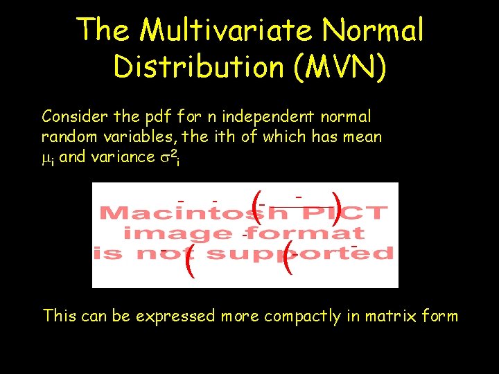
The Multivariate Normal Distribution (MVN) Consider the pdf for n independent normal random variables, the ith of which has mean mi and variance s 2 i - ( - ) - This can be expressed more compactly in matrix form

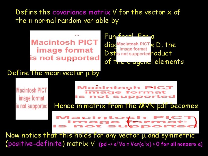
Define the covariance matrix V for the vector x of the n normal random variable by … Fun fact! For a diagonal matrix D, the Det = | D | = product of the diagonal elements … Define the mean vector m by - - Hence in matrix from the MVN pdf becomes - - ( - - ) Now notice that this holds for any vector m and symmetric (positive-definite) matrix V (pd -> a. TVa = Var(a. Tx) > 0 for all nonzero a)

Properties of the MVN - I 1) If x is MVN, any subset of the variables in x is also MVN 2) If x is MVN, any linear combination of the elements of x is also MVN. If x is MVN(m, V) ( )

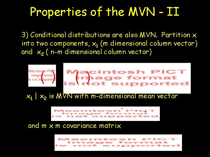
Properties of the MVN - II 3) Conditional distributions are also MVN. Partition x into two components, x 1 (m dimensional column vector) and x 2 ( n-m dimensional column vector) ( ) x 1 | x 2 is MVN with m-dimensional mean vector - - and m x m covariance matrix - -

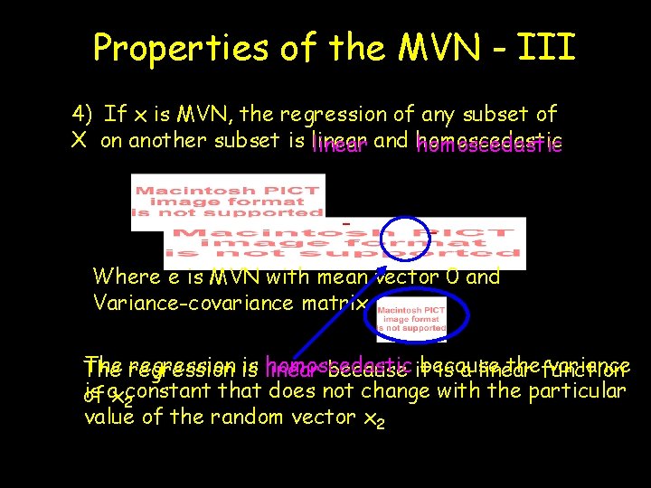
Properties of the MVN - III 4) If x is MVN, the regression of any subset of X on another subset is linear and homoscedastic - - Where e is MVN with mean vector 0 and Variance-covariance matrix The regression is is linear homoscedastic because thefunction variance The because it is a linear is ax 2 constant that does not change with the particular of value of the random vector x 2

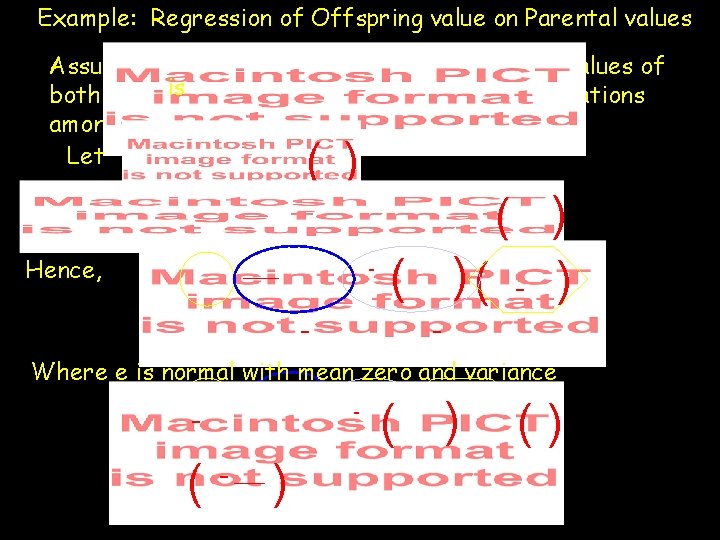
Example: Regression of Offspring value on Parental values Assume the vector of offspring value and the values of is both its parents is MVN. Then from the correlations among (outbred) relatives, Let ( ) Hence, - - ( )( - ) - Where e is normal with mean zero and variance - ( ) ( - ) ()

Hence, the regression of offspring trait value given the trait values of its parents is zo = mo + h 2/2(zs- ms) + h 2/2(zd- md) + e where the residual e is normal with mean zero and Var(e) = sz 2(1 -h 4/2) Similar logic gives the regression of offspring breeding value on parental breeding value as Ao = mo + (As- ms)/2+ (Ad- md)/2 + e = As/2+ Ad/2 + e where the residual e is normal with mean zero and Var(e) = s. A 2/2

Lecture 10 b: Linear Models

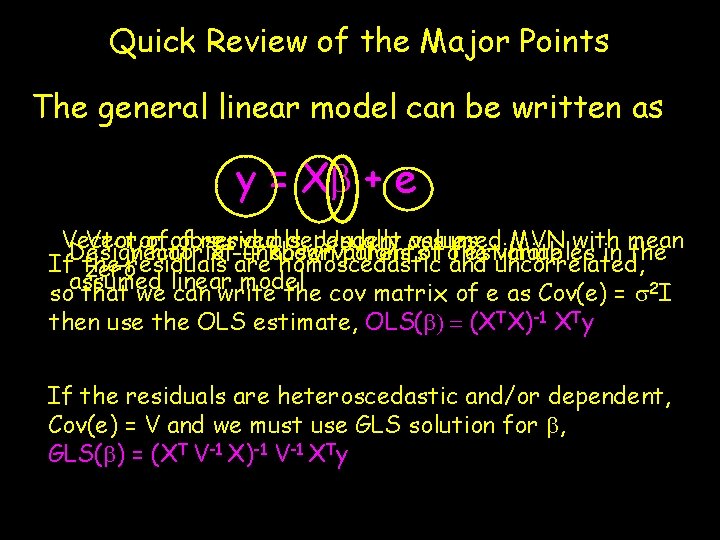
Quick Review of the Major Points The general linear model can be written as y = Xb + e Vector of residuals. Usually assumed MVN with mean Vector of observed dependent values Vector of--unknown parents tothe estimate Design matrix observations of variables in the If the residuals are homoscedastic and uncorrelated, zero linear model assumed so that we can write the cov matrix of e as Cov(e) = s 2 I then use the OLS estimate, OLS(b) = (XTX)-1 XTy If the residuals are heteroscedastic and/or dependent, Cov(e) = V and we must use GLS solution for b, GLS(b) = (XT V-1 X)-1 V-1 XTy

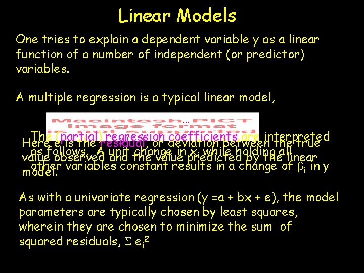
Linear Models One tries to explain a dependent variable y as a linear function of a number of independent (or predictor) variables. A multiple regression is a typical linear model, … The (partial) regression coefficients are interpreted Here e is the residual, or deviation between the true as follows. A unit change in xi while holding all value observed and the value predicted by the linear other variables constant results in a change of bi in y model. As with a univariate regression (y =a + bx + e), the model parameters are typically chosen by least squares, wherein they are chosen to minimize the sum of squared residuals, S ei 2

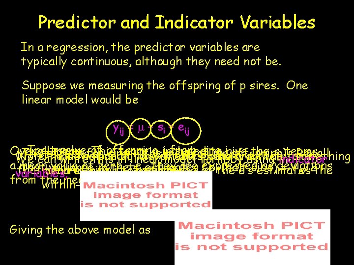
Predictor and Indicator Variables In a regression, the predictor variables are typically continuous, although they need not be. Suppose we measuring the offspring of p sires. One linear model would be yij = m + si + eij Trait valuefor of offspring jincluded from of sire igive Overall mean. This term invariables to the s isterms The effect sire i (the mean its offspring). Recall Note The that deviation the predictor of the jth offspring here from are the , something We can write this in linear model form by using indicator ifamily a that mean value of zero, i. e. , they are of expressed as deviations that variance in the s estimates Cov(half sibs) = VA/2 the mean we are of trying sire i. to The estimate i variance the e’s estimates variables, from the mean within-family variance. Giving the above model as

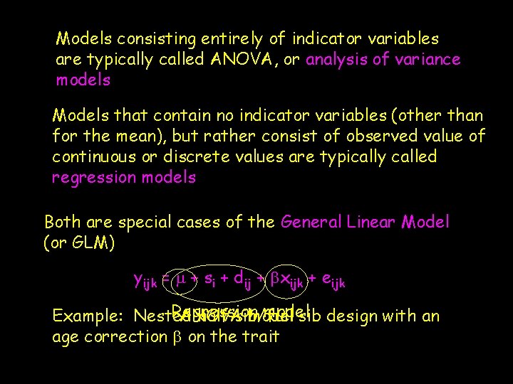
Models consisting entirely of indicator variables are typically called ANOVA, or analysis of variance models Models that contain no indicator variables (other than for the mean), but rather consist of observed value of continuous or discrete values are typically called regression models Both are special cases of the General Linear Model (or GLM) yijk = m + si + dij + bxijk + eijk Regression model ANOVA model Example: Nested half sib/full sib design with an age correction b on the trait

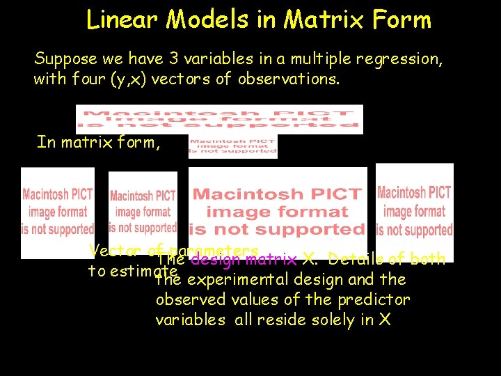
Linear Models in Matrix Form Suppose we have 3 variables in a multiple regression, with four (y, x) vectors of observations. In matrix form, Vector of parameters The design matrix X. Details of both to estimate the experimental design and the observed values of the predictor variables all reside solely in X

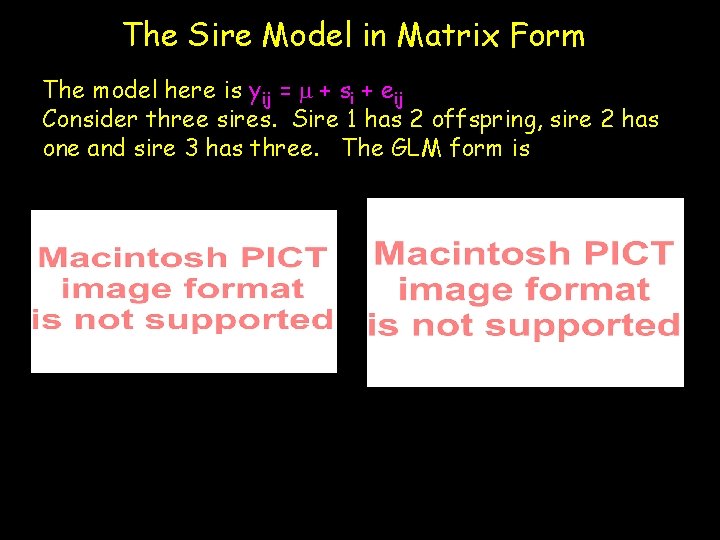
The Sire Model in Matrix Form The model here is yij = m + si + eij Consider three sires. Sire 1 has 2 offspring, sire 2 has one and sire 3 has three. The GLM form is

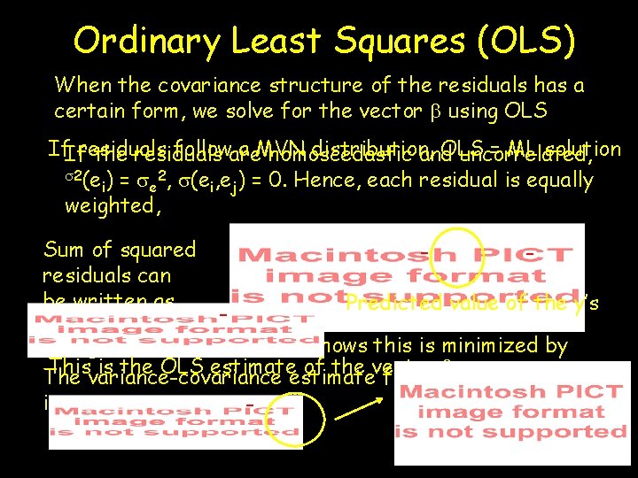
Ordinary Least Squares (OLS) When the covariance structure of the residuals has a certain form, we solve for the vector b using OLS If. Ifresiduals followare a MVN distribution, OLS = ML solution the residuals homoscedastic and uncorrelated, s 2(e ) = s 2, s(e , e ) = 0. Hence, each residual is equally i e i j weighted, Sum of squared residuals can be written as - - Predicted value of the y’s Taking (matrix) derivatives shows this is minimized by Thisvariance-covariance is the OLS estimate of the vector b sample estimates The for the is -

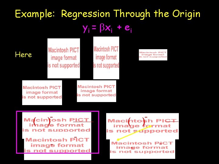
Example: Regression Through the Origin yi = bxi + ei Here ( - ) - ( - - ) -

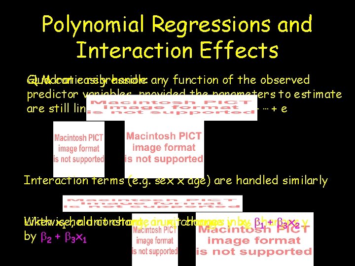
Polynomial Regressions and Interaction Effects GLM can easily handle any function of the observed Quadratic regression: predictor variables, provided the parameters to estimate are still linear, e. g. Y = a +b 1 f(x) + b 1 g(x) + … + e Interaction terms (e. g. sex x age) are handled similarly With x 1 held constant, change in x 2 bchanges Likewise, a unit change ainunit x 1 changes y by 1 + b 3 x 2 y by b 2 + b 3 x 1

Fixed vs. Random Effects In linear models are trying to accomplish two goals: estimation the values of model parameters and estimate any appropriate variances. For example in the simplest regression model, y = a + bx + e, we estimate the values for a and b and also the variance of e. We, of course, can also estimate the ei = yi - (a + bxi ) Note that a/b are fixed constants are we trying to estimate (fixed factors or fixed effects), while the ei values are drawn from some probability distribution (typically Normal with mean 0, variance s 2 e). The ei are random effects.

This distinction between fixed and random effects is extremely important in terms of how we analyzed a model. If a parameter is a fixed constant we wish to estimate, it is a fixed effect. If a parameter are drawn from some probability distribution and we are trying to make inference on either the distribution and/or specific realizations from this distribution, it is a random effect. We generally speak of estimating fixed factors and predicting random effects. “Mixed” models contain both fixed and random factors

Example: Sire model yij = m + si + eij It Conversely, depends. Is the sire if Ifwe effect we Fixed are have not fixed effect (say) Random only or 10 interested random? sires, effect if we in these are ONLY interested 10 particular in the sires values but also of these wish to particular make some 10 sires and don’t inference care to about make the any population other inferences from which about they the population were drawn from (such which as theadditive sires are variance, drawn, then sincewe can treat s 2 A =them 4 s 2 s, as ), then fixedthe effects. si are random In the effects. case, the In model thisis fully case specified we wish tothe estimate covariance m andstructure the variances for the residuals. 2. Since Thus, s 2 s and wesneed to estimate 2 si also m, estimates s 1 to s 10 (or andpredicts) s 2 e, and we w 2 wish write the breeding the model value as for yij =sire m + si, i we + ealso s 2 e. ij, s (e ij) =to estimate (predict) these as well. Under a Random-effects interpretation, we write the model as yij = m + si + eij, s 2(eij) = s 2 e, s 2(si) = s 2 s

Generalized Least Squares (GLS) Suppose the residuals no longer have the same variance (i. e. , display heteroscedasticity). Clearly we do not wish to minimize the unweighted sum of squared residuals, because those residuals with smaller variance should receive more weight. Likewise in the event the residuals are correlated, we also wish to take this into account (i. e. , perform a suitable transformation to remove the correlations) before minimizing the sum of squares. Either of the above settings leads to a GLS solution in place of an OLS solution.

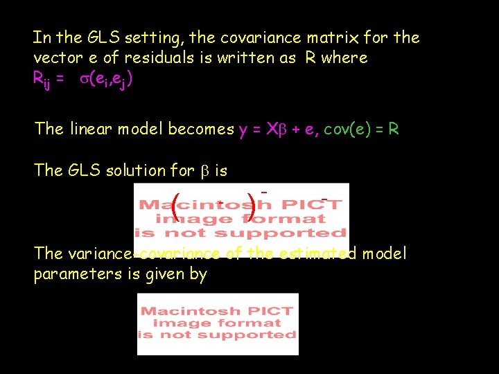
In the GLS setting, the covariance matrix for the vector e of residuals is written as R where Rij = s(ei, ej) The linear model becomes y = Xb + e, cov(e) = R The GLS solution for b is ( ) - - - The variance-covariance of the estimated model parameters is given by ( - ) -

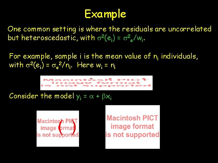
Example One common setting is where the residuals are uncorrelated but heteroscedastic, with s 2(ei) = s 2 e/wi. For example, sample i is the mean value of n i individuals, with s 2(ei) = se 2/ni. Here wi = ni - - Consider the model yi = a + bxi ( ) -

Here giving where -

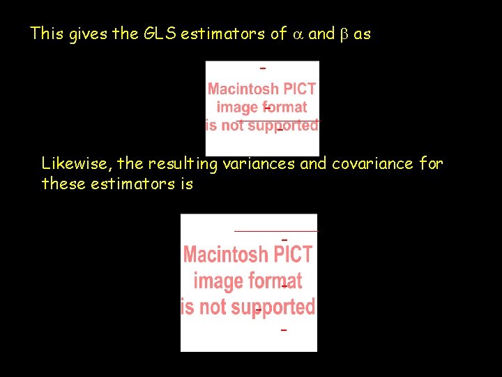
This gives the GLS estimators of a and b as - - Likewise, the resulting variances and covariance for these estimators is - - -