Lecture 1 Introduction to Managerial Economics Professor Information

Lecture 1 Introduction to Managerial Economics

Professor Information • Current and previous academic appointments • Hankamer School of Business, Baylor University: Professor of Finance and Insurance (2000 -Present) and Frank S. Groner Memorial Chair of Finance (2002 Present) • The Wharton School of the University of Pennsylvania: Visiting Scholar (2007 -present) • Previous faculty appointments at Penn State (19841989), UT-Austin (1989 -1996), LSU (1998 -2000), and Wharton (Spring 2006 Semester) Business Schools 2 • Research: Application of economics and finance to the analysis, pricing, and management of risk. • Service: Associate editor of two journals: Geneva Risk and Insurance Review and Journal of Risk and Insurance; Past President of two academic associations: American Risk and Insurance Lecture 1: Introduction to Managerial Economics

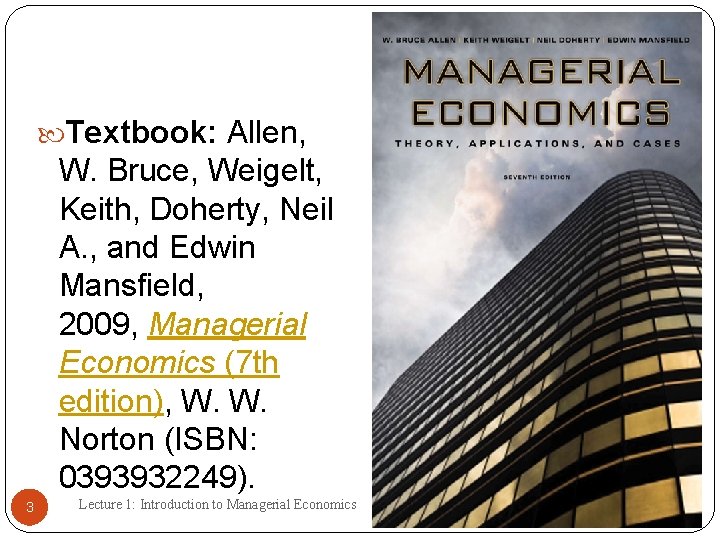
Textbook: Allen, W. Bruce, Weigelt, Keith, Doherty, Neil A. , and Edwin Mansfield, 2009, Managerial Economics (7 th edition), W. W. Norton (ISBN: 0393932249). 3 Lecture 1: Introduction to Managerial Economics

Course Goals Learn to use economic models to think critically 4 about everyday problems. Know what conditions characterize competitive outcomes and efficient allocations of resources. Understand how firm cost structure and the nature of the market determine prices and production; learn how firms with pricing power can exploit variation in demand to price discriminate and maximize profits. Apply strategic thinking to decision-making and know how to use it to analyze firm and individual choices. Lecture 1: Introduction tohow Managerial Economics Understand risk influences decision-making

Grade Determination Final Grade =. 30(Problem Sets) + . 30(Midterm Exam 1) +. 40(Final Exam) The midterm exam will occur in class on Thursday, November 5. The final exam will occur during the final class session on Monday, December 14. 5 Lecture 1: Introduction to Managerial Economics

Microeconomics and Macroeconomics Microeconomics represents the branch 6 of economics which deals with the behavior of individual economic units— consumers, firms, workers, and investors—as well as the markets that these units comprise. Macroeconomics represents the branch of economics which deals with aggregate economic variables, such as the level and growth rate of national Lecture 1: Introductioninterest to Managerial Economics output, rates, unemployment,

Managerial Economics Managerial economics involves the application of microeconomics to analyze managerial actions and their effect on firm performance. The purpose of this analysis is to shed 7 light on concepts such as cost, demand, profit, competition, pricing, compensation, and business strategy. With its focus on behavior, managerial economics provides powerful tools and Lecture 1: Introduction to Managerial Economics frameworks to guide managers to better

Business and the Social Sciences Economics, psychology, and sociology represent the “parent” social sciences upon which most business disciplines are based. Managerial economics, finance and accounting draw primarily on economics (especially micro), whereas management and marketing tend to be based primarily upon psychology and sociology. Counterexamples include behavioral economics and finance, 8 use of econ-based pricing strategies in marketing, application game theory in management strategy, etc. Lectureof 1: Introduction to Managerial Economics

Managerial Economics Where does managerial economics fit within the EMBA curriculum? Managerial economics is a standard first- 9 year course requirement in most EMBA programs. This course differs conceptually from other first-year courses in that it (like QBA 5330) focuses upon the analytic foundations for decision-making that are subsequently applied in “core business Lecture 1: Introduction to Managerial Economics

Internet Resources • Class website: http: //economics. garven. com • The source for readings, lecture notes, problem sets, etc. • For links requiring authentication, use “econ” as your username and “baylor” as your password (all lowercase). • Class weblog: http: //econblog. garven. com 10 • Lecture I use thetoclass blog to post important 1: Introduction Managerial Economics

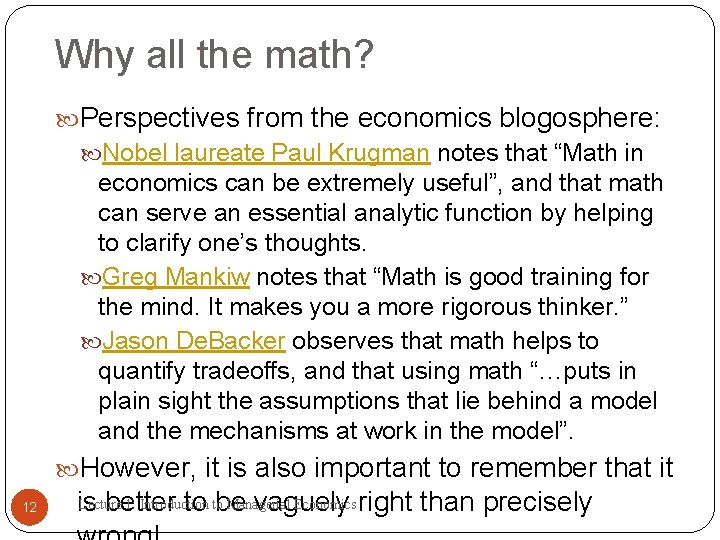
Why all the math? Perspective from the great master, Alfred Marshall: 11 In a letter to his protégée, A. C. Pigou, he [Marshall] laid out the following system: “(1) Use mathematics as shorthand language, rather than as an engine of inquiry. (2) Keep to them till you have done. (3) Translate into English. (4) Then illustrate by examples that are important in real life (5) Burn the mathematics. (6) If you can’t succeed in 4, burn 3. Thisto Managerial I do often. ” Lecture 1: Introduction Economics

Why all the math? Perspectives from the economics blogosphere: Nobel laureate Paul Krugman notes that “Math in economics can be extremely useful”, and that math can serve an essential analytic function by helping to clarify one’s thoughts. Greg Mankiw notes that “Math is good training for the mind. It makes you a more rigorous thinker. ” Jason De. Backer observes that math helps to quantify tradeoffs, and that using math “…puts in plain sight the assumptions that lie behind a model and the mechanisms at work in the model”. However, it is also important to remember that it 12 Lecture 1: Introduction Managerial Economics right than precisely is better to tobe vaguely

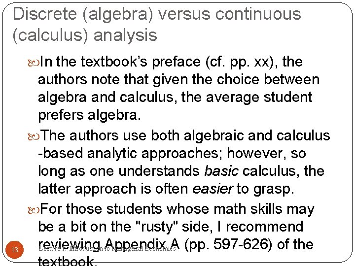
Discrete (algebra) versus continuous (calculus) analysis In the textbook’s preface (cf. pp. xx), the 13 authors note that given the choice between algebra and calculus, the average student prefers algebra. The authors use both algebraic and calculus -based analytic approaches; however, so long as one understands basic calculus, the latter approach is often easier to grasp. For those students whose math skills may be a bit on the "rusty" side, I recommend reviewing A (pp. 597 -626) of the Lecture 1: Introduction Appendix to Managerial Economics

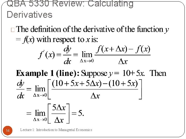
QBA 5330 Review: Calculating Derivatives 14 Lecture 1: Introduction to Managerial Economics

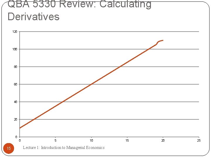
QBA 5330 Review: Calculating Derivatives 120 100 80 60 40 20 0 0 15 5 10 Lecture 1: Introduction to Managerial Economics 15 20 25

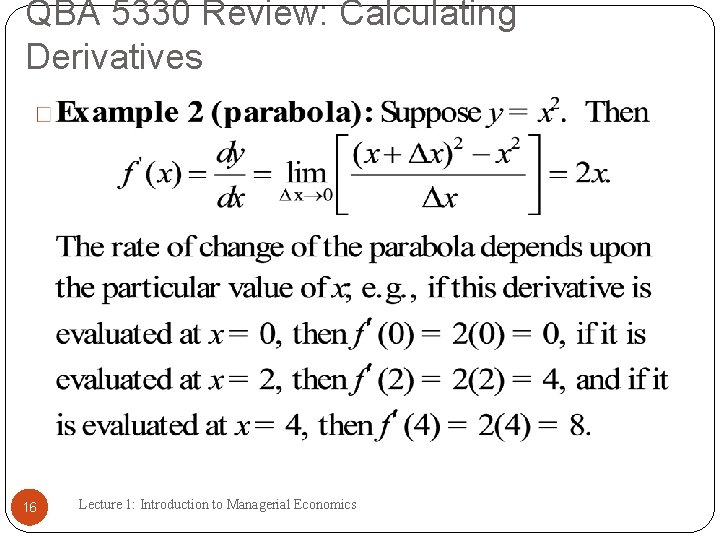
QBA 5330 Review: Calculating Derivatives 16 Lecture 1: Introduction to Managerial Economics

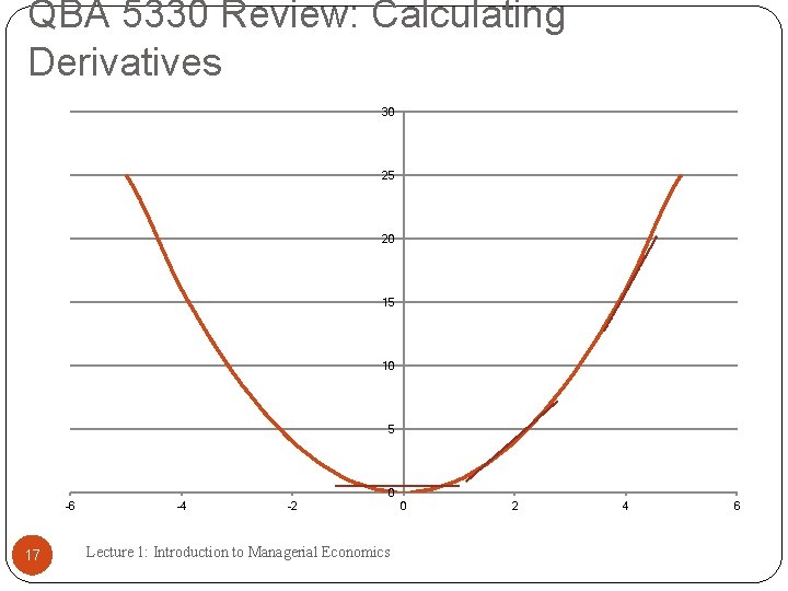
QBA 5330 Review: Calculating Derivatives 30 25 20 15 10 5 0 -6 17 -4 -2 Lecture 1: Introduction to Managerial Economics 0 2 4 6

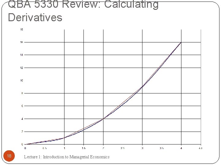
QBA 5330 Review: Calculating Derivatives 18 Lecture 1: Introduction to Managerial Economics

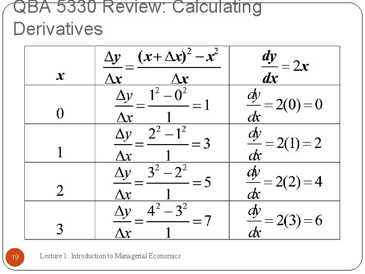
QBA 5330 Review: Calculating Derivatives 19 Lecture 1: Introduction to Managerial Economics

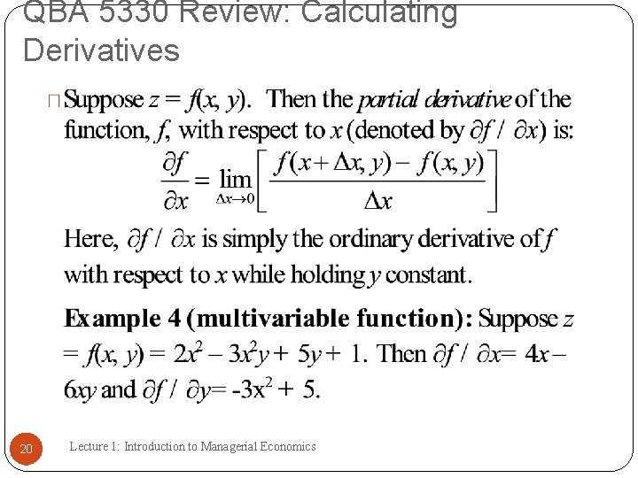
QBA 5330 Review: Calculating Derivatives 20 Lecture 1: Introduction to Managerial Economics

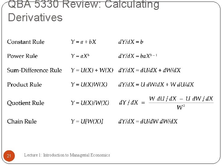
QBA 5330 Review: Calculating Derivatives 21 Lecture 1: Introduction to Managerial Economics

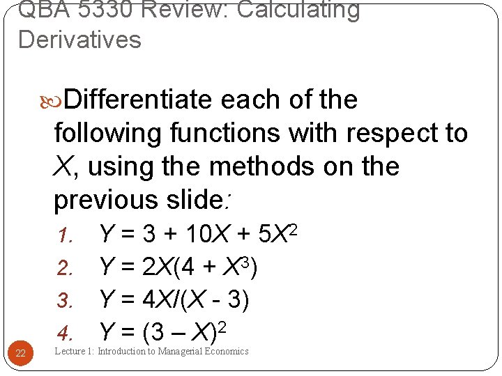
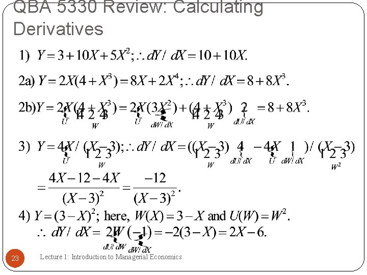
QBA 5330 Review: Calculating Derivatives Differentiate each of the following functions with respect to X, using the methods on the previous slide: Y = 3 + 10 X + 5 X 2 2. Y = 2 X(4 + X 3) 3. Y = 4 X/(X - 3) 4. Y = (3 – X)2 1. 22 Lecture 1: Introduction to Managerial Economics

QBA 5330 Review: Calculating Derivatives 23 Lecture 1: Introduction to Managerial Economics

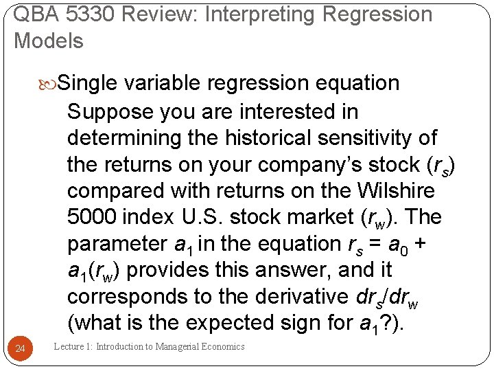
QBA 5330 Review: Interpreting Regression Models Single variable regression equation Suppose you are interested in determining the historical sensitivity of the returns on your company’s stock (rs) compared with returns on the Wilshire 5000 index U. S. stock market (rw). The parameter a 1 in the equation rs = a 0 + a 1(rw) provides this answer, and it corresponds to the derivative drs/drw (what is the expected sign for a 1? ). 24 Lecture 1: Introduction to Managerial Economics

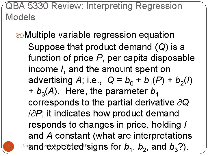
QBA 5330 Review: Interpreting Regression Models Multiple variable regression equation 25 Suppose that product demand (Q) is a function of price P, per capita disposable income I, and the amount spent on advertising A; i. e. , Q = b 0 + b 1(P) + b 2(I) + b 3(A). Here, the parameter b 1 corresponds to the partial derivative ¶Q /¶P; it indicates how product demand responds to changes in price, holding I and A constant (what are interpretations Lecture 1: Introduction to Managerial Economics and expected signs for b 1, b 2, and b 3? ).

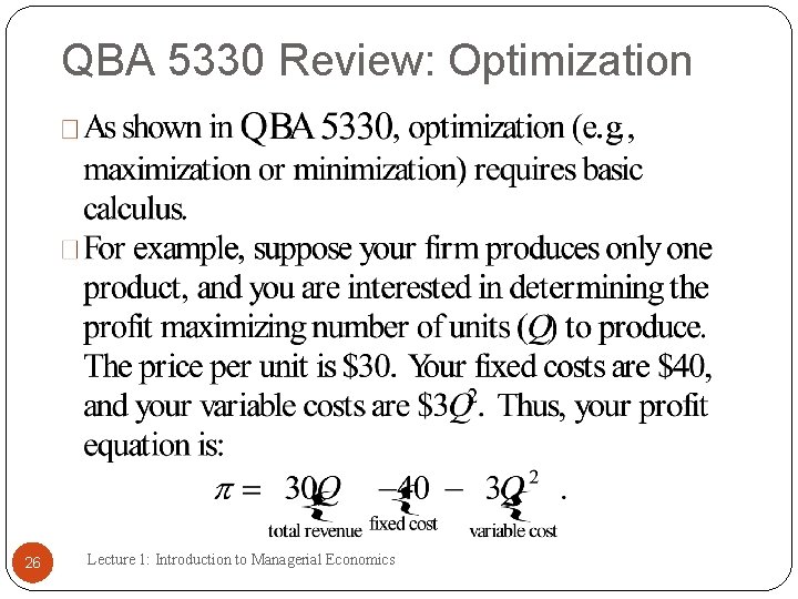
QBA 5330 Review: Optimization 26 Lecture 1: Introduction to Managerial Economics

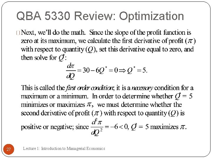
QBA 5330 Review: Optimization 27 Lecture 1: Introduction to Managerial Economics

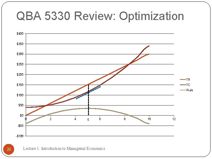
QBA 5330 Review: Optimization $400 $350 $300 $250 $200 TR $150 TC Profit $100 $50 $0 0 2 4 5 6 -$50 -$100 28 Lecture 1: Introduction to Managerial Economics 8 10 12

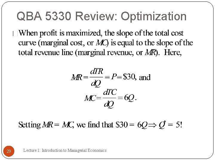
QBA 5330 Review: Optimization 29 Lecture 1: Introduction to Managerial Economics

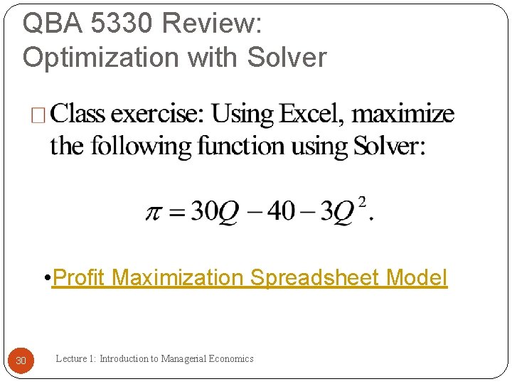
QBA 5330 Review: Optimization with Solver • Profit Maximization Spreadsheet Model 30 Lecture 1: Introduction to Managerial Economics

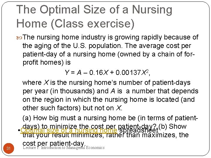
The Optimal Size of a Nursing Home (Class exercise) The nursing home industry is growing rapidly because of 31 the aging of the U. S. population. The average cost per patient-day of a nursing home (owned by a chain of forprofit homes) is Y = A – 0. 16 X + 0. 00137 X 2, where X is the nursing home’s number of patient-days per year (in thousands) and A is a number that depends on the region in which the nursing home is located (and other such factors) but not on X. (a) How big must a nursing home be (in terms of patientdays) to minimize the cost per patient-day? (b) Show • Optimal size of a nursing home spreadsheet that your result minimizes, rather than maximizes, the cost per patient-day. Lecture 1: Introduction to Managerial Economics

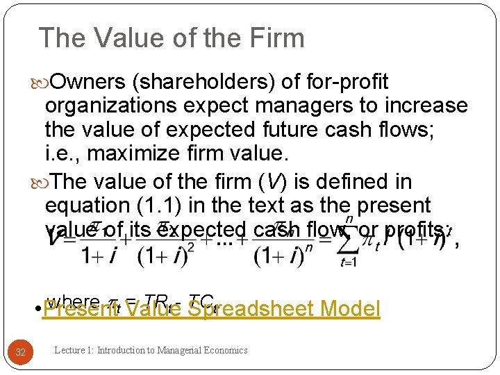
The Value of the Firm Owners (shareholders) of for-profit organizations expect managers to increase the value of expected future cash flows; i. e. , maximize firm value. The value of the firm (V) is defined in equation (1. 1) in the text as the present value of its expected cash flow, or profits: where pt Value = TRt - TC t. • Present Spreadsheet Model 32 Lecture 1: Introduction to Managerial Economics

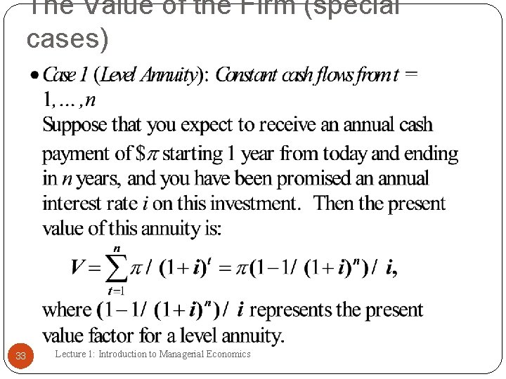
The Value of the Firm (special cases) 33 Lecture 1: Introduction to Managerial Economics

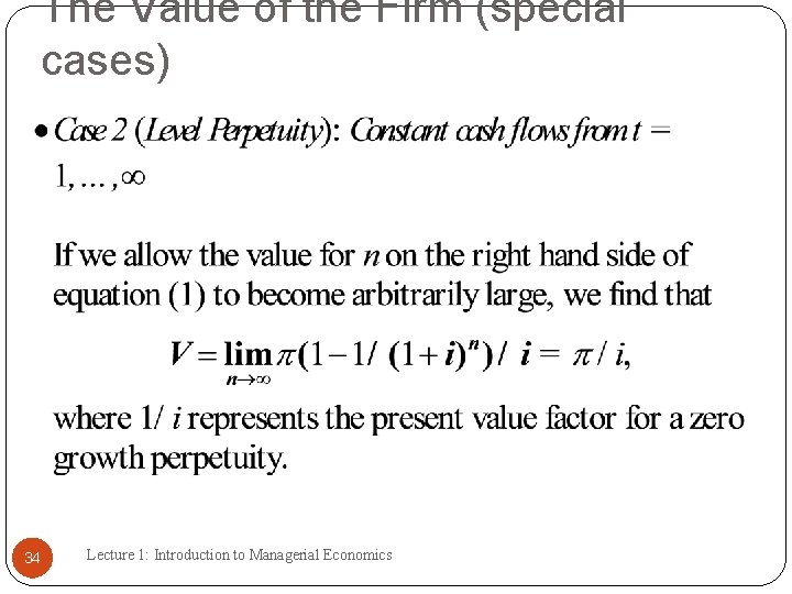
The Value of the Firm (special cases) 34 Lecture 1: Introduction to Managerial Economics

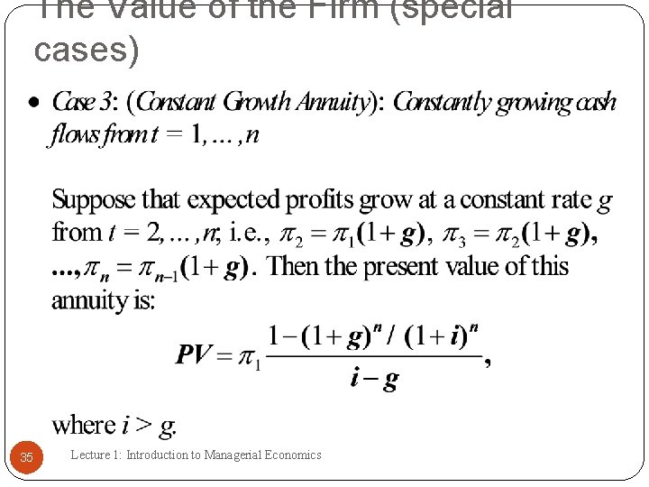
The Value of the Firm (special cases) 35 Lecture 1: Introduction to Managerial Economics

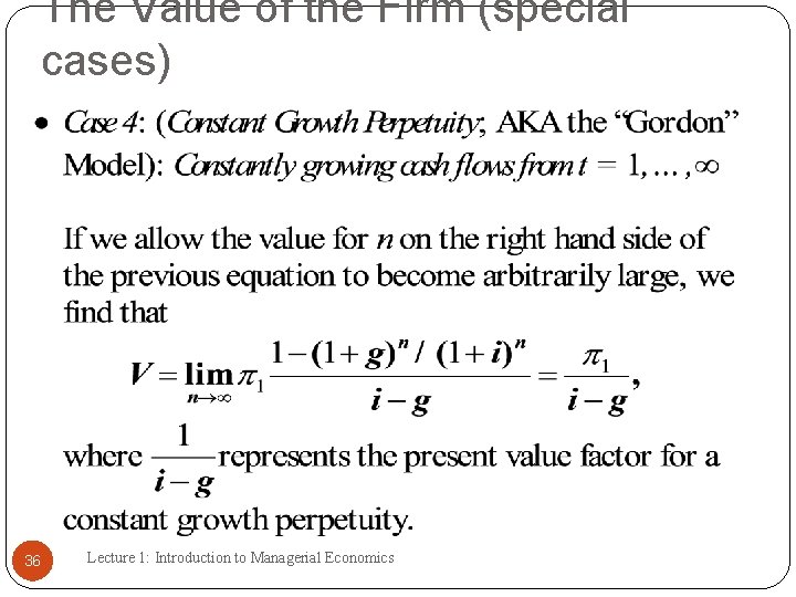
The Value of the Firm (special cases) 36 Lecture 1: Introduction to Managerial Economics

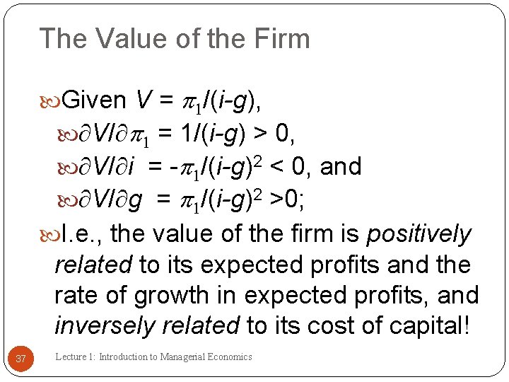
The Value of the Firm Given V = p 1/(i-g), ¶V/¶p 1 = 1/(i-g) > 0, ¶V/¶i = -p 1/(i-g)2 < 0, and ¶V/¶g = p 1/(i-g)2 >0; I. e. , the value of the firm is positively related to its expected profits and the rate of growth in expected profits, and inversely related to its cost of capital! 37 Lecture 1: Introduction to Managerial Economics

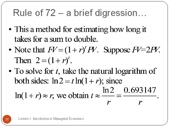
Rule of 72 – a brief digression… 38 Lecture 1: Introduction to Managerial Economics

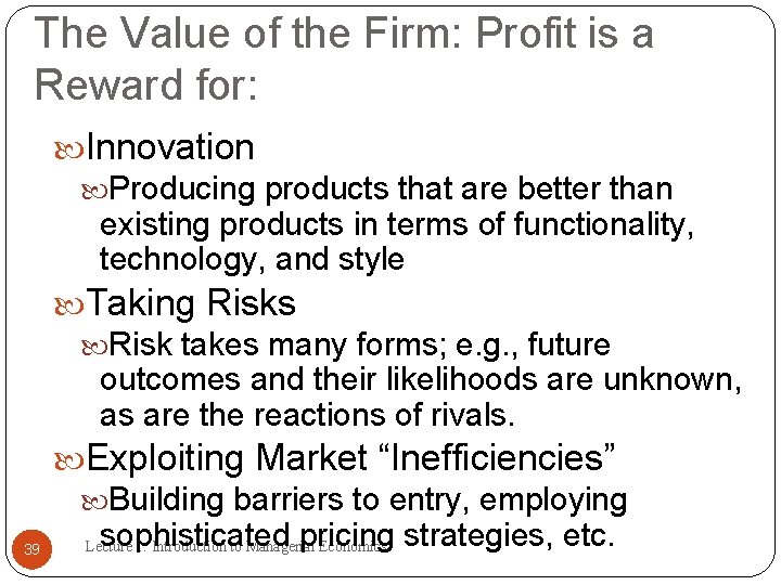
The Value of the Firm: Profit is a Reward for: 39 Innovation Producing products that are better than existing products in terms of functionality, technology, and style Taking Risks Risk takes many forms; e. g. , future outcomes and their likelihoods are unknown, as are the reactions of rivals. Exploiting Market “Inefficiencies” Building barriers to entry, employing sophisticated pricing Lecture 1: Introduction to Managerial Economics strategies, etc.

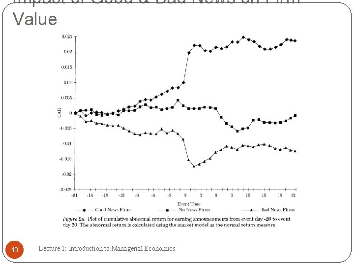
Impact of Good & Bad News on Firm Value 40 Lecture 1: Introduction to Managerial Economics

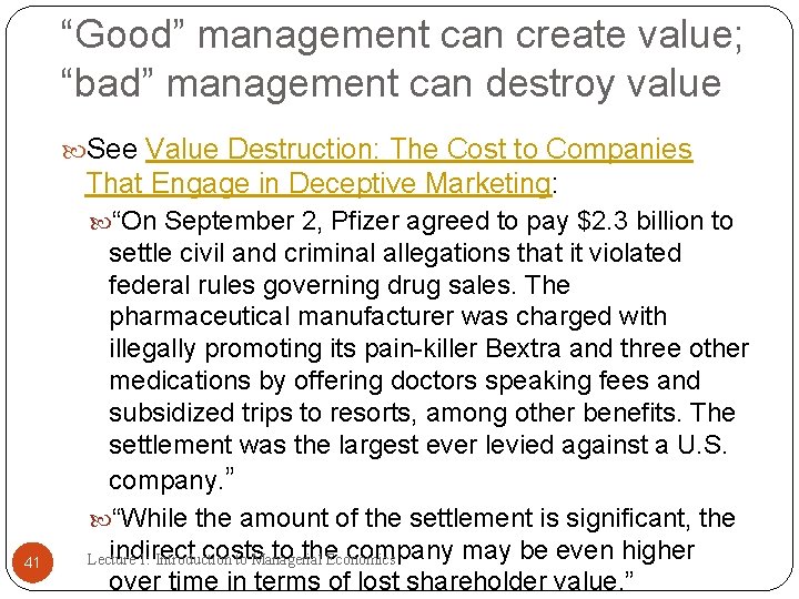
“Good” management can create value; “bad” management can destroy value See Value Destruction: The Cost to Companies That Engage in Deceptive Marketing: “On September 2, Pfizer agreed to pay $2. 3 billion to 41 settle civil and criminal allegations that it violated federal rules governing drug sales. The pharmaceutical manufacturer was charged with illegally promoting its pain-killer Bextra and three other medications by offering doctors speaking fees and subsidized trips to resorts, among other benefits. The settlement was the largest ever levied against a U. S. company. ” “While the amount of the settlement is significant, the indirect costs to the. Economics company may be even higher Lecture 1: Introduction to Managerial over time in terms of lost shareholder value. ”

The Principal-Agent Problem Managerial Interests and the Principal-Agent Problem The interests of a firm's owners and 42 those of its managers may diverge, unless the manager is the owner. However, the separation of ownership and control is often necessary because the capital raising and risk bearing capabilities of Lecture 1: Introduction to Managerial Economics entrepreneurs are limited.

The Principal-Agent Problem Separation of ownership and control The principals are the owners. They want managers to maximize firm value. The agents are the managers. Other things equal, they prefer more compensation and less accountability. The divergence in goals is 43 commonly referred to as the principal-agent problem. Lecture 1: Introduction to Managerial Economics

Moral Hazard A moral hazard occurs when one party is 44 responsible for the interests of another, but has an incentive to put his or her own interests first. If I can take risks that you have to bear, then I may as well take them; however, if I have to bear the consequences of my risky actions, this will motivate me to act more prudently. Managers who choose not to maximize Lecture 1: Introduction to Managerial Economics firm value may act this way if

Solution: Moral Hazard Devise methods that lead to 45 convergence of the interests of the firm's owners and its managers Examples: contract design which ties managerial compensation to shareholder welfare; e. g. , via share/option ownership, bonuses Lecture 1: Introduction to Managerial Economics

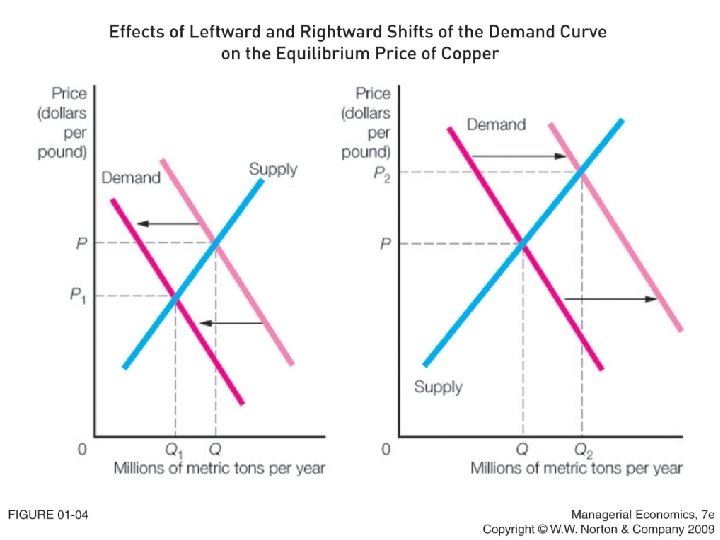
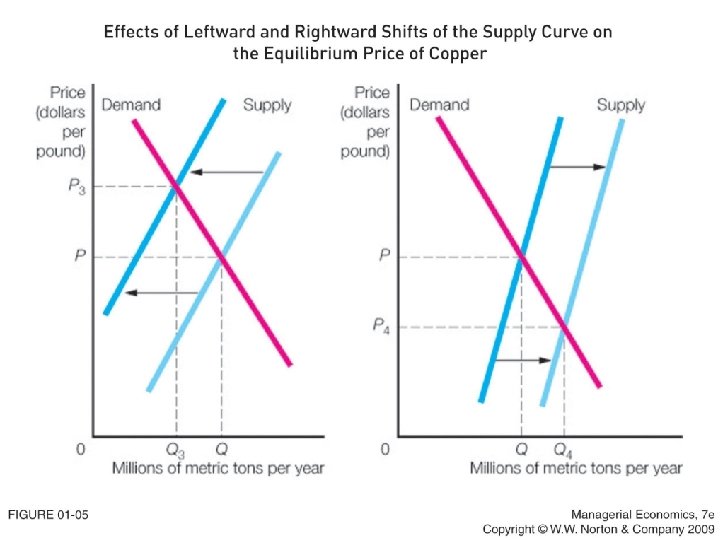
Demand Supply: a First Look A market exists when there is 46 economic exchange; that is, individuals and organizations interact with each other to buy or sell goods and services. Markets typically function well so long as contracts are binding and enforceable, which in turn implies respect for the rule of law and Lecture 1: Introduction to Managerial Economics

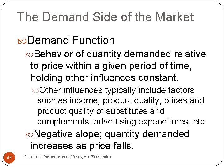
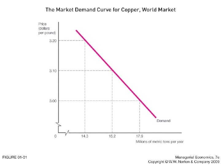
The Demand Side of the Market Demand Function Behavior of quantity demanded relative to price within a given period of time, holding other influences constant. Other influences typically include factors such as income, product quality, prices and product quality of substitutes and complements, advertising expenditures, etc. Negative slope; quantity demanded increases as price falls. 47 Lecture 1: Introduction to Managerial Economics

48

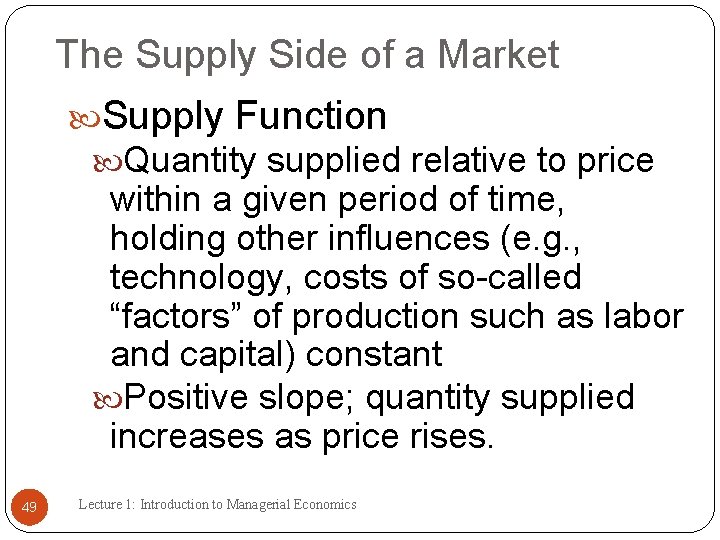
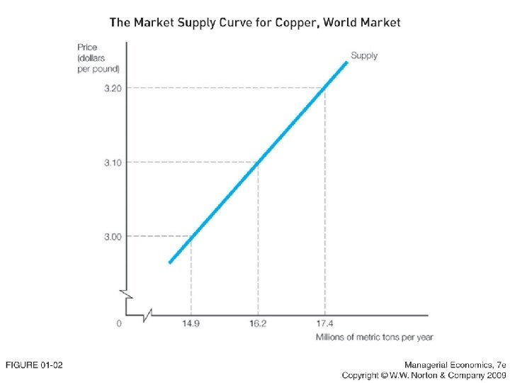
The Supply Side of a Market Supply Function Quantity supplied relative to price within a given period of time, holding other influences (e. g. , technology, costs of so-called “factors” of production such as labor and capital) constant Positive slope; quantity supplied increases as price rises. 49 Lecture 1: Introduction to Managerial Economics

50

51

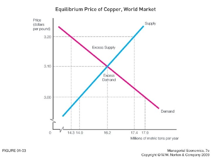
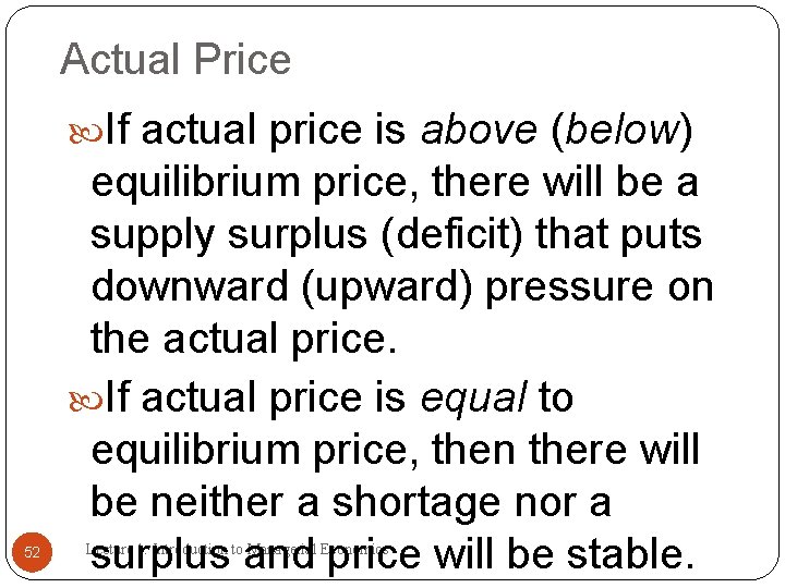
Actual Price If actual price is above (below) 52 equilibrium price, there will be a supply surplus (deficit) that puts downward (upward) pressure on the actual price. If actual price is equal to equilibrium price, then there will be neither a shortage nor a surplus and price will be stable. Lecture 1: Introduction to Managerial Economics

53

54