Lecture 1 Historical Timeline in Nuclear Medicine Mathematics

Lecture 1 Ø Historical Timeline in Nuclear Medicine ØMathematics Review Ø Image of the week

Mathematical Review • Graphs • Continous vs. Discrete Functions • Geometry • Exponential Functions • Trigonometry • Scientific Notation • Significant Figures

Graphical Operations Number Line Ø one dimensional Ø infinite in + and - directions

Number Line Ø A ruler is a number line Ø measuring height of individuals

2 -Dimensional Coordinates Y = ex

Sudden earthquake activity

Expanded Earthquake Graph

Another 2 D Example e-x**2

3 Dimensional Coordinates

Three Dimensional Graph e-(x**2 + y**2)

Three dimensional display

Continuous Function

Discrete Function

Discrete function “Approximates” Continuous Function

Nuclear Medicine Example

DATA x=time 1 2 3 4 5 6 7 8 9 10 11 y 1 = x**2 1 4 9 16 25 36 49 64 81 100 121 y 2 = x**3 1 8 27 64 125 216 343 512 729 1000 1331

Y = X 2 AND Y = X 3

Geometry Area of rectangle

Volume of box V=lxwxh

Right triangle Area = ?

The circle Area = pi x r 2

Trigonometry The Navigation Problem

Graphing Data Another Way Sine and Cosine waves

Periodic function

Model of Shape of Electromagnetic Radiation “Wave Function”

Periodic Wave Function

Exponential Functions 1 • Functions of the type ex, e-ax, eiΘ, e-x 2, ex 2 • • • have many applications in science. We will study e-ax , e-x 2 and equations derived from these. Some physical processes exhibit “exponential” behavior. Some examples are attenuation of photon radiation, and radioactive decay.

Exponential Functions e-x

Normal Distribution e-x**2

Scientific Notation • Used with constants such as velocity of light: • 3. 0 x 1010 cm/sec Simplifies writing numbers: 3. 0 x 1010 100000 = 300000. = 3 x

Rule for scientific notation: n x = n zeros x-n = n – 1 zeros

Proportions • Direct Proportion: Y = k * X • If k = 1, X = Y • Inverse Proportion: Y = k/X • If k = 1, Y = 1/X • * means multiplication

Examples Ø Ø Attenuation and Dose Calculations Inverse square law Effective half life Discrete image representation

The Attenuation Equation • Given a beam containing a large flux of monoenergetic photons, and a uniform absorber, the removal (attenuation) of photons from the beam can be described as an exponential process.

• • • The equation which describes this process is: I = I 0 x e-ux Where, I = Intensity remaining I 0 = initial photon intensity x = thickness of absorber u = constant that determines the attenuation of the photons, and, therefore, the shape of the exponential function.

• Experimental data demonstrates that • μ = 0. 693/ HVL, where HVL stands for Half Value Layer and represents that thickness of absorber material which reduces I to one/half its value. μ is called the linear attenuation coefficient and is a parameter which is a “constant” of attenuation for a given HVL

Derivation • If we interposed increasing thickness of absorbers between a source of photons and a detector, we would obtain this graph.

The line through the data points is a mathematical determination which best describes the measured points. The equation describes an exponential process

Variables • The value of HVL depends on the energy of • • the photons, and type of absorber. For a given absorber, the higher the photon energy, the lower the HVL. For a given photon energy, the higher the atomic number of the absorber, the higher the HVL.

Example 1 • The HVL of lead for 140 Ke. V photons is: • • 0. 3 mm What is u? 0. 693/0. 3 = 2. 31 cm-1

Example 2 Given the data in Example 1, what % of photons are detected after a thickness of 0. 65 mm are placed between the source and detector? Solution: using I = I 0 x e-ux, with I 0 = 100, u = 2. 31 cm-1, x= 0. 65, and solving for I, I = 22%

Decay Equation: A = A 0 x e-lambda x t Where, A = Activity remaining A 0 = Initial Activity t = elapsed time u = constant that determines the decay of the radioactive sample, and, therefore, the shape of the exponential function.

• Experimental data demonstrates that lambda = 0. 693/ Half Life where Half Life represents the time it takes for a sample to decay to 50% of it’s value.

Example 1 A dose of FDG is assayed as 60 m. Ci/1. 3 ml, at 8 AM You need to administer a dose of 20 m. Ci at 1 PM. How much volume should you draw into the syringe? • • • First, identify the terms: A =? t. =5 Ao =60 T/12 = 1. 8 hrs We see that A is the unknown. Then, inserting the values into the equation, we have: A = 60 x exp(0. 693/1. 8) x 5) A = 8. 8 m. Ci So at 1 PM you have 8. 8 m. Ci/1. 3 ml. You need to draw up 20/8. 8 = 2. 27 times the volume needed 5 hours ago. This amounts to 2. 27 x 1. 3 = 3 ml

Example 2: A cyclotron operator needs to irradiate enough H 2 O to be able to supply the radiochemist with 500 m. Ci/ml F-18 at 3 PM. The operator runs the cyclotron at 8: 30 AM. How much activity/ml is needed at that time? • • • • There are really two ways that we can solve this. The first, and easier way: Write: Ao = Ax(exp(λt ) Notice we have a positive exponent. In other words, instead of using the law of decay, use the law of growth Once again, identify the terms, and the unknown: A = 500 T = 6. 5 Ao = ? T/12 = 1. 8 hrs Exchange Ao and A Ao = A x (exp(λt ) A = 500 x (exp(0. 693/1. 8 x 6. 5) A = 6106 m. Ci at 8: 30 AM. = 6. 106 Ci

• • The second way: A = Ao x exp(-λt ) = 500 x (exp(-0. 693/1. 8 x 6. 5) 500 = Ao x exp(-(2. 5025) 500 = Ao = 6106 m. Ci = 6. 106 Ci 0. 08

Effective Half Life • 1/Te = 1/Tb + 1/Tp • Where Te = Effective Half Life • Tb = biological half life • Tp = physical half life

Inverse Square Law • The intensity of Radiation from a point source is inversely proportional to the square of the distance • I 1/I 2 = D 22 / D 12

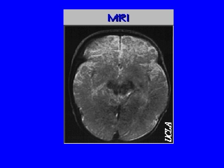
Image of the Week

This digital image is a 2 dimensional graph. Why?

Lecture 2, January 18 • • Licenses and Regulatory Authorities Authorized Users Radiation Safety Officer Emergency Contacts