Lecture 1 Basic Statistical Tools Discrete and Continuous

Lecture 1: Basic Statistical Tools

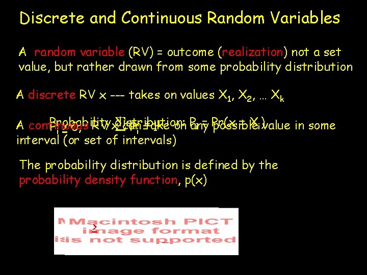
Discrete and Continuous Random Variables A random variable (RV) = outcome (realization) not a set value, but rather drawn from some probability distribution A discrete RV x --- takes on values X 1, X 2, … Xk S Probability = Xi)value in some A continuous can i = Pr(x possible Pi > 0, RV xdistribution: Pi =take 1 on Pany interval (or set of intervals) The probability distribution is defined by the probability density function, p(x) <> <

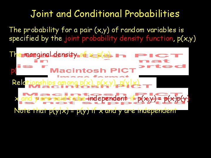
Joint and Conditional Probabilities The probability for a pair (x, y) of random variables is specified by the joint probability density function, p(x, y) The marginal density of x, p(x) < < p(y|x), the conditional density y given x Relationships among p(x), p(x, y), p(y|x) < < x and y are said to be independent if p(x, y) = p(x)p(y) Note that p(y|x) = p(y) if x and y are independent

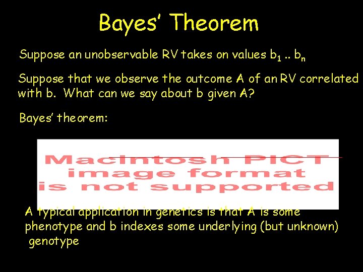
Bayes’ Theorem Suppose an unobservable RV takes on values b 1. . bn Suppose that we observe the outcome A of an RV correlated with b. What can we say about b given A? Bayes’ theorem: A typical application in genetics is that A is some phenotype and b indexes some underlying (but unknown) genotype

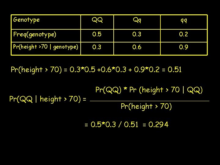
Genotype QQ Qq qq Freq(genotype) 0. 5 0. 3 0. 2 Pr(height >70 | genotype) 0. 3 0. 6 0. 9 Pr(height > 70) = 0. 3*0. 5 +0. 6*0. 3 + 0. 9*0. 2 = 0. 51 Pr(QQ | height > 70) = Pr(QQ) * Pr (height > 70 | QQ) Pr(height > 70) = 0. 5*0. 3 / 0. 51 = 0. 294

Expectations of Random Variables The expected value, E [f(x)], of some function x of the random variable x is just the average value of that function E[x] = the (arithmetic) mean, m, of a random variable x x discrete x continuous E[ (x - m)2 ] = s 2, the variance of x More generally, the rth moment about the mean is given ] [ by E[ (x - m)r ] Useful properties expectations r ==2: =3: 4: variance skew (scaled)ofkurtosis

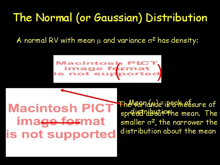
The Normal (or Gaussian) Distribution A normal RV with mean m and variance s 2 has density: ( ) (m) =ispeak of The. Mean variance a measure of distribution spread about the mean. The smaller s 2, the narrower the distribution about the mean

The truncated normal Only consider values of T or above in a normal Density = distribution p(x | x > T) Mean of function truncated Here p. T is the height of the normal Variance at the truncation point, T Let p. T = Pr(z > T)

Covariances • Cov(x, y) = E [(x-mx)(y-my)] • = E [x*y] - E[x]*E[y] Cov(x, y) >=<0, 0, negative (linear) association between Cov(x, y) = 0 linear DOES NOTassociation imply no association Cov(x, y) 0, positive no association between x & y x x&&y y

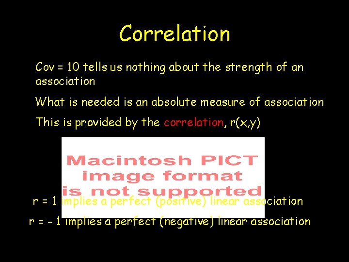
Correlation Cov = 10 tells us nothing about the strength of an association What is needed is an absolute measure of association This is provided by the correlation, r(x, y) r = 1 implies a perfect (positive) linear association r = - 1 implies a perfect (negative) linear association

Useful Properties of Variances and Covariances • Symmetry, Cov(x, y) = Cov(y, x) • The covariance of a variable with itself is the variance, Cov(x, x) = Var(x) • If a is a constant, then – Cov(ax, y) = a Cov(x, y) • Var(a x) = a 2 Var(x). – Var(ax) = Cov(ax, ax) = a 2 Cov(x, x) = a 2 Var(x) • Cov(x+y, z) = Cov(x, z) + Cov(y, z)

More generally Hence, the variance of a sum equals the sum of the Variances ONLY when the elements are uncorrelated

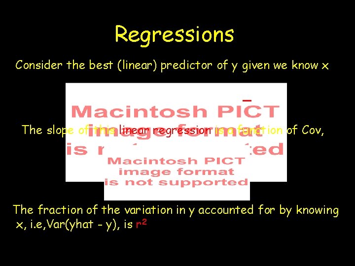
Regressions Consider the best (linear) predictor of y given we know x The slope of this linear regression is a function of Cov, The fraction of the variation in y accounted for by knowing x, i. e, Var(yhat - y), is r 2

Relationship between the correlation and the regression Slope: If Var(x) = Var(y), then by|x = b x|y = r(x, y) In the case, the fraction of variation accounted for by the regression is b 2

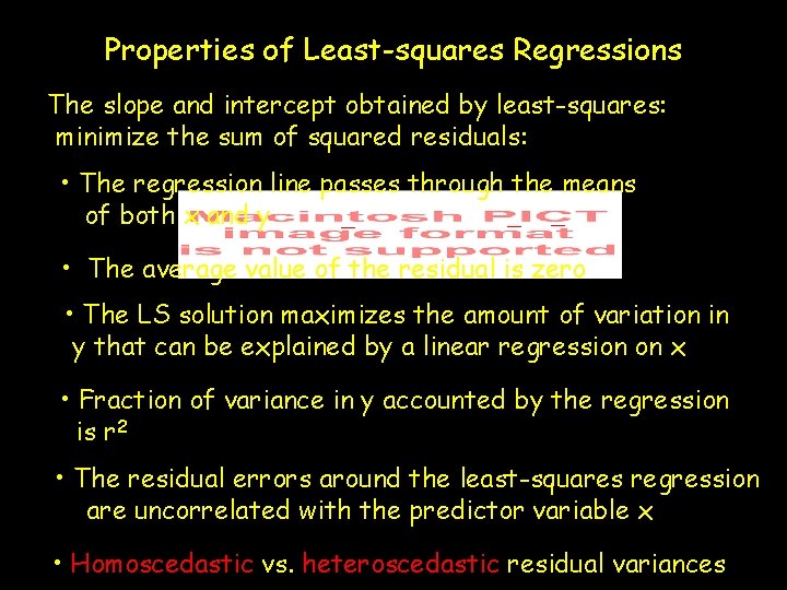
Properties of Least-squares Regressions The slope and intercept obtained by least-squares: minimize the sum of squared residuals: • The regression line passes through the means of both x and y • The average value of the residual is zero • The LS solution maximizes the amount of variation in y that can be explained by a linear regression on x • Fraction of variance in y accounted by the regression is r 2 • The residual errors around the least-squares regression are uncorrelated with the predictor variable x • Homoscedastic vs. heteroscedastic residual variances

Maximum Likelihood p(x 1, …, xn | q ) = density of the observed data (x 1, …, xn) given the (unknown) distribution parameter(s) q Fisher (yup, the same one) suggested the method of maximum likelihood --- given the data (x 1, …, xn) find the value(s) of q that maximize p(x 1, …, xn | q ) We usually express p(x 1, …, xn | q) as a likelihood function l ( q | x 1, …, xn ) to remind us that it is dependent on the observed data The Maximum Likelihood Estimator (MLE) of q are the value(s) that maximize the likelihood function l given the observed data x 1, …, xn.

MLE of q l (q | x) This curvature The is formalize of by thelooking likelihood at the surface log-likelihood in the neighborhood surface, of=the L ln [l. MLE (q | informs x) ]. Since us as lnto is the a monotonic precisionfunction, of the estimator the A narrow value of q peak that =maximizes high precision. l also maximizes A board peak L = lower precision Var(MLE) = -1 Negative curvature larger the curvature, the smaller at a maximum The 2 nd derivative = curvature the variance

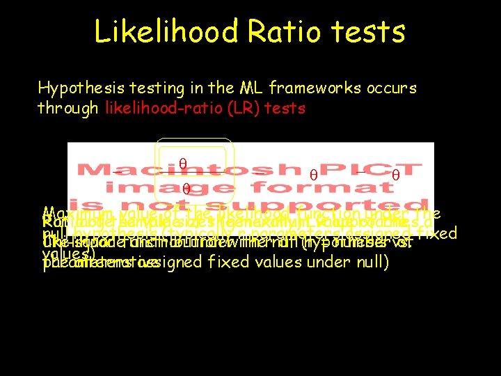
Likelihood Ratio tests Hypothesis testing in the ML frameworks occurs through likelihood-ratio (LR) tests q q Maximum value of the likelihood function under the Ratio For large of the sample valuesizes of the (generally) maximum. LR value approaches of the a null hypothesis (typically r parameters assigned fixed likelihood function Chi-square distribution underwith thernull df (r hypothesis = numbervs. of values) the alternative parameters assigned fixed values under null)

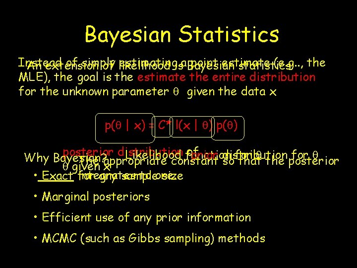
Bayesian Statistics Instead of simply estimatingisa. Bayesian point estimate (e. g. . , the An extension of likelihood statistics MLE), the goal is the estimate the entire distribution for the unknown parameter q given the data x p(q | x) = C* l(x | q) p(q) posterior distribution of Likelihood function prior distribution for q Why Bayesian? The appropriate constant so that the posterior q given x integrates to one. • Exact for any sample size • Marginal posteriors • Efficient use of any prior information • MCMC (such as Gibbs sampling) methods