Lecture 05 Consumer Preferences and the Concept of

Lecture # 05 Consumer Preferences and the Concept of Utility (cont. ) Lecturer: Martin Paredes

Indifference Curves (end) 2. The Marginal Rate of Substitution 3. The Utility Function l Marginal Utility 4. Some Special Functional Forms 1. 2

Definition: An Indifference Curve is the set of all baskets for which the consumer is indifferent Definition: An Indifference Map illustrates the set of indifference curves for a particular consumer 3

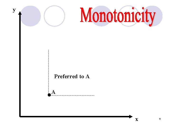
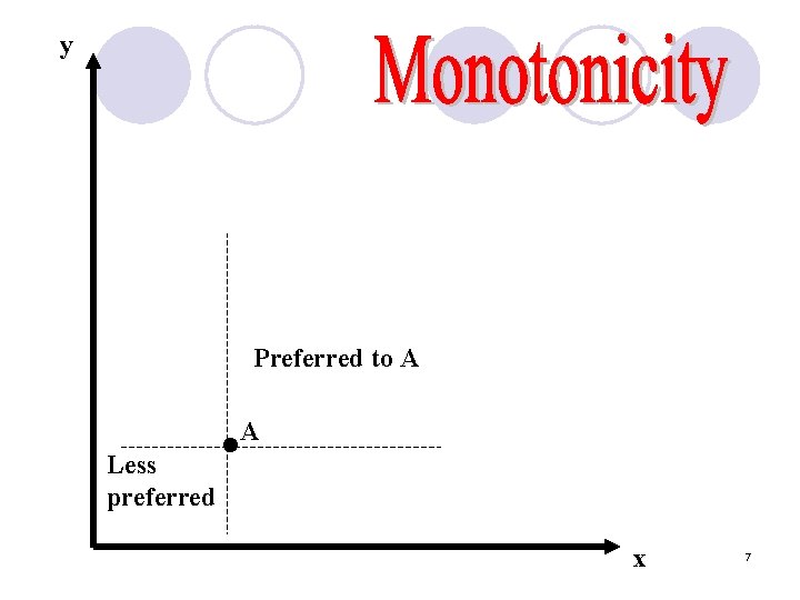
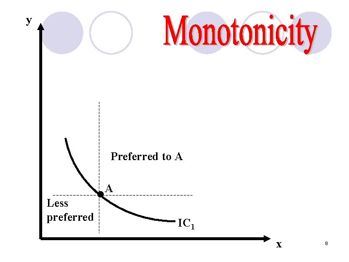
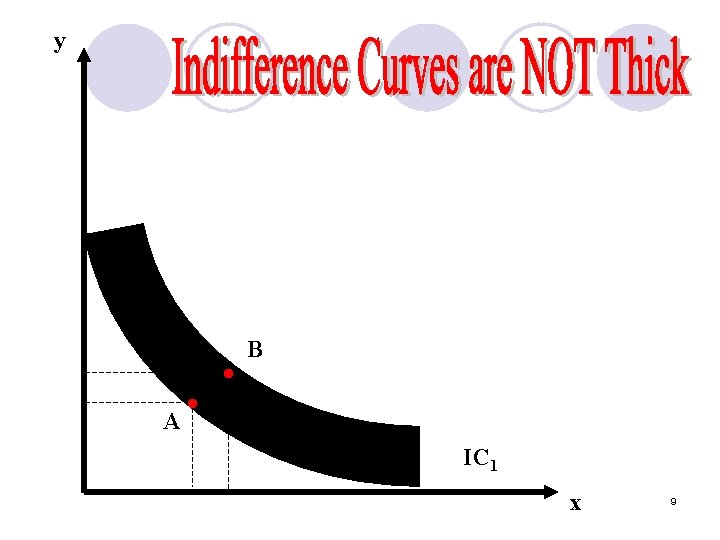
1. Completeness l Each basket lies on only one indifference curve 2. Monotonicity l Indifference curves have negative slope l Indifference curves are not “thick” 4

y • A x 5

y Preferred to A • A x 6

y Preferred to A • A Less preferred x 7

y Preferred to A • A Less preferred IC 1 x 8

y A • • B IC 1 x 9

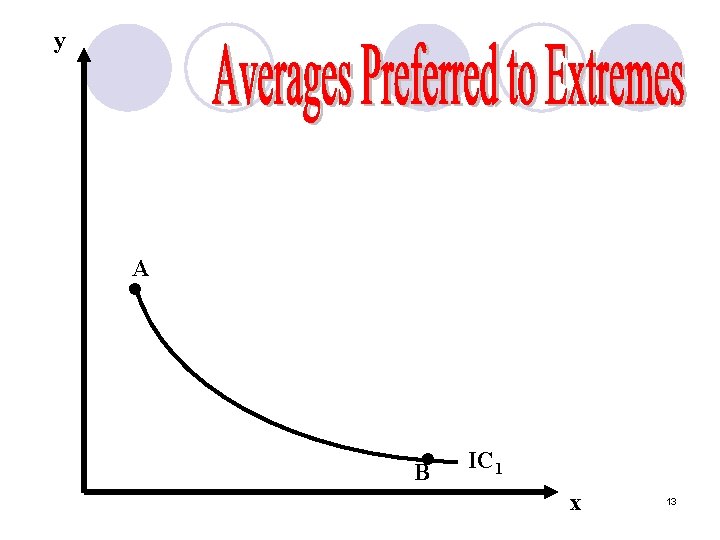
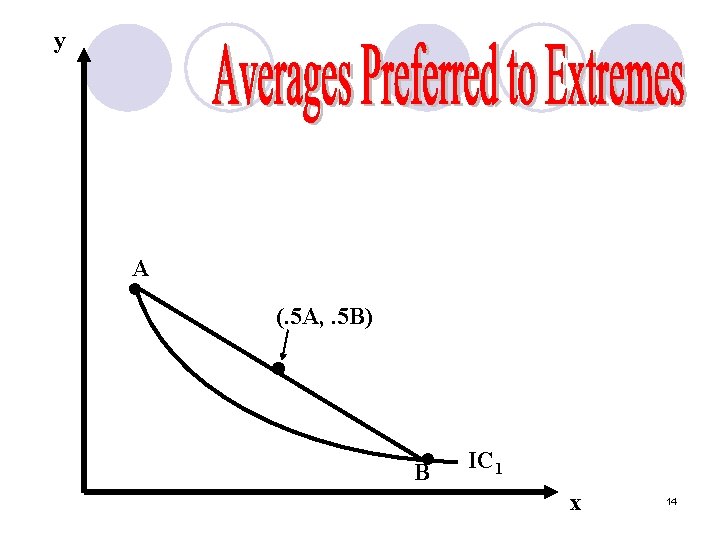
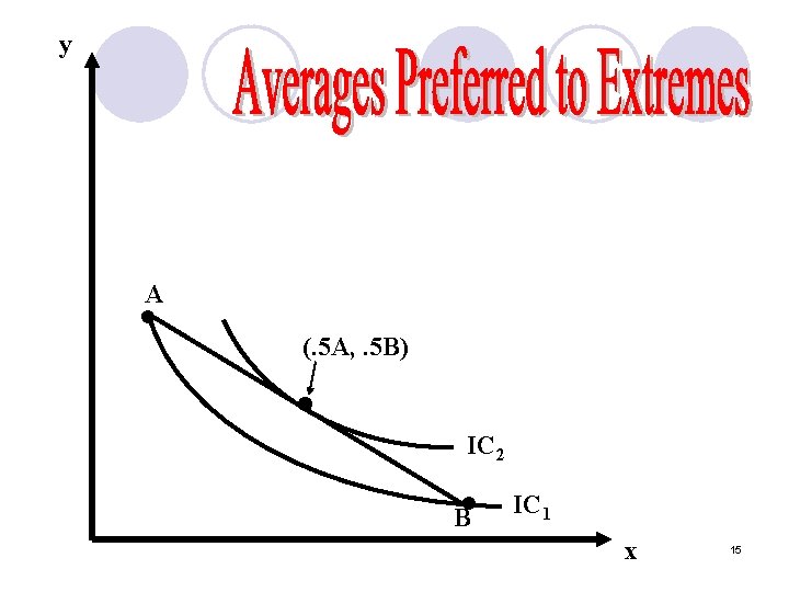
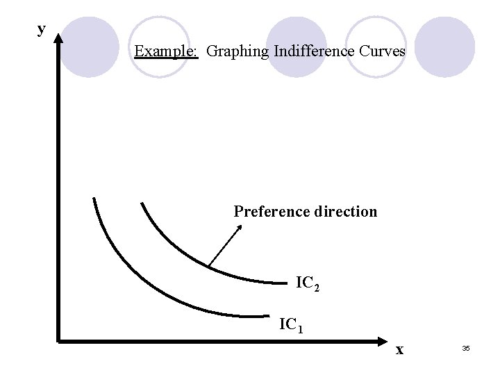
3. Transitivity l Indifference curves do not cross 4. Averages preferred to extremes l Indifference curves are bowed toward the origin (convex to the origin). 10

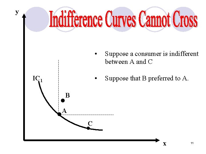
y IC 1 • Suppose a consumer is indifferent between A and C • Suppose that B preferred to A. B • A • C • x 11

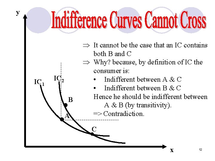
y IC 1 IC 2 B • A • Þ It cannot be the case that an IC contains both B and C Þ Why? because, by definition of IC the consumer is: • Indifferent between A & C • Indifferent between B & C Hence he should be indifferent between A & B (by transitivity). => Contradiction. C • x 12

y A • • B IC 1 x 13

y A • (. 5 A, . 5 B) • IC 2 • B IC 1 x 15

There are several ways to define the Marginal Rate of Substitution Definition 1: It is the maximum rate at which the consumer would be willing to substitute a little more of good x for a little less of good y in order to leave the consumer just indifferent between consuming the old basket or the new basket 16

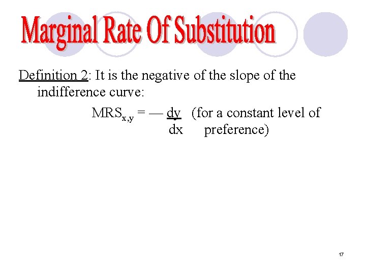
Definition 2: It is the negative of the slope of the indifference curve: MRSx, y = — dy (for a constant level of dx preference) 17

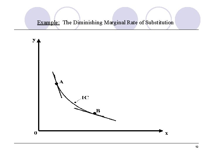
An indifference curve exhibits a diminishing marginal rate of substitution: 1. The more of good x you have, the more you are willing to give up to get a little of good y. 2. The indifference curves • Get flatter as we move out along the horizontal axis • Get steeper as we move up along the vertical axis. 18

Example: The Diminishing Marginal Rate of Substitution 19

Definition: The utility function measures the level of satisfaction that a consumer receives from any basket of goods. 20

l The utility function assigns a number to each basket l More preferred baskets get a higher number than less preferred baskets. l Utility is an ordinal concept l The precise magnitude of the number that the function assigns has no significance. 21

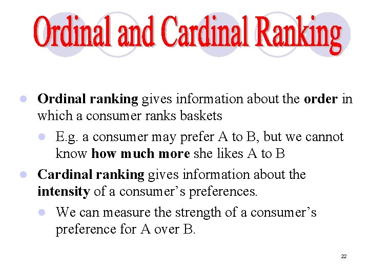
Ordinal ranking gives information about the order in which a consumer ranks baskets l E. g. a consumer may prefer A to B, but we cannot know how much more she likes A to B l Cardinal ranking gives information about the intensity of a consumer’s preferences. l We can measure the strength of a consumer’s preference for A over B. l 22

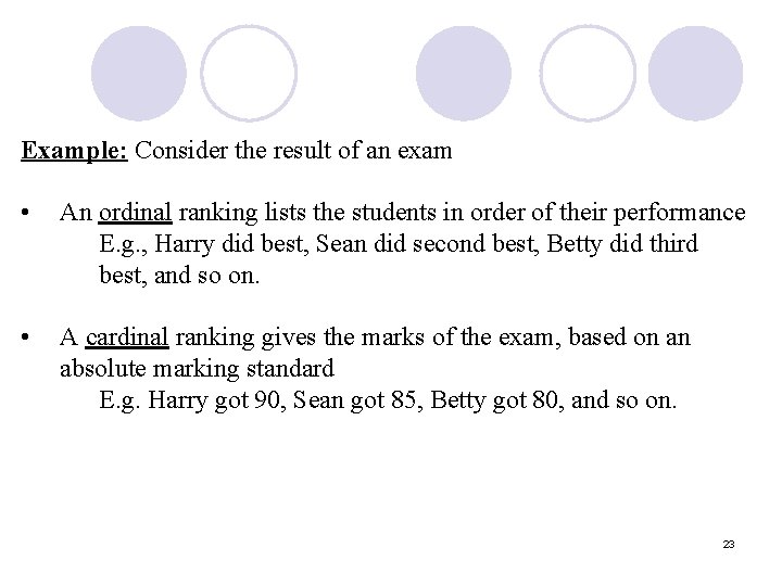
Example: Consider the result of an exam • • An ordinal ranking lists the students in order of their performance E. g. , Harry did best, Sean did second best, Betty did third best, and so on. A cardinal ranking gives the marks of the exam, based on an absolute marking standard E. g. Harry got 90, Sean got 85, Betty got 80, and so on. 23

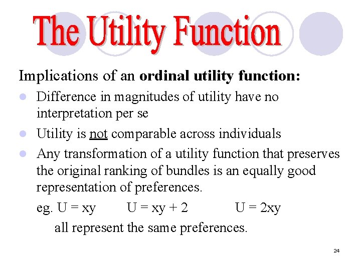
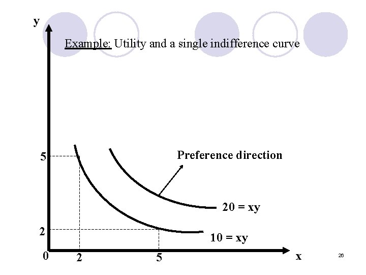
Implications of an ordinal utility function: Difference in magnitudes of utility have no interpretation per se l Utility is not comparable across individuals l Any transformation of a utility function that preserves the original ranking of bundles is an equally good representation of preferences. eg. U = xy + 2 U = 2 xy all represent the same preferences. l 24

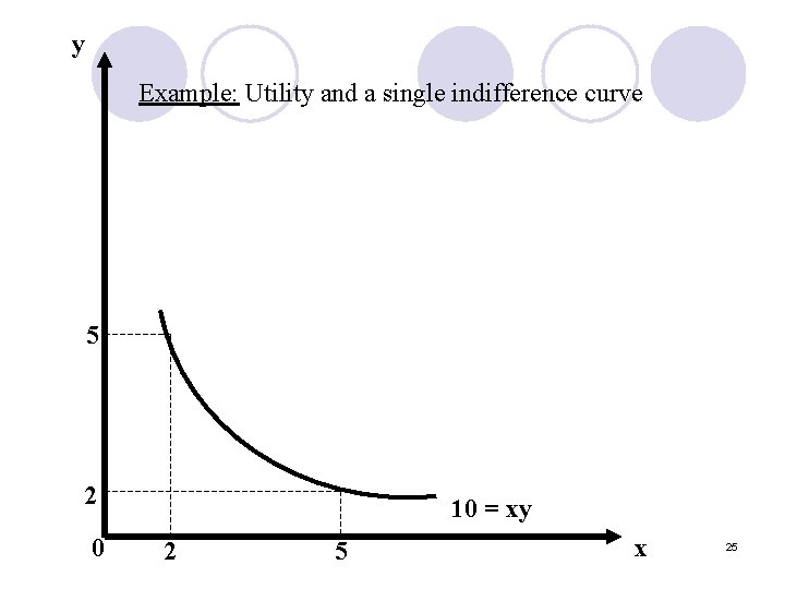
y Example: Utility and a single indifference curve 5 2 0 10 = xy 2 5 x 25

y Example: Utility and a single indifference curve Preference direction 5 20 = xy 2 0 10 = xy 2 5 x 26

Definition: The marginal utility of good x is the additional utility that the consumer gets from consuming a little more of x MUx = d. U dx l It is is the slope of the utility function with respect to x. l It assumes that the consumption of all other goods in consumer’s basket remain constant. 27

Definition: The principle of diminishing marginal utility states that the marginal utility of a good falls as consumption of that good increases. Note: A positive marginal utility implies monotonicity. 28

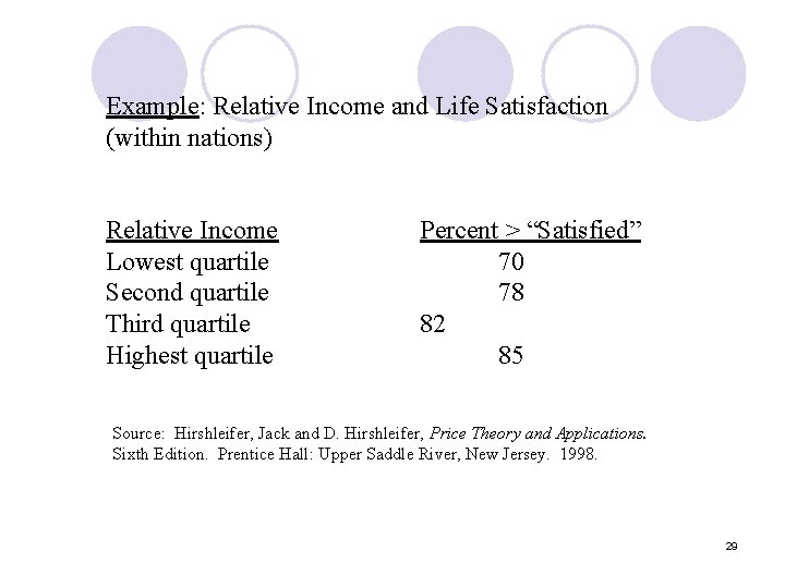
Example: Relative Income and Life Satisfaction (within nations) Relative Income Lowest quartile Second quartile Third quartile Highest quartile Percent > “Satisfied” 70 78 82 85 Source: Hirshleifer, Jack and D. Hirshleifer, Price Theory and Applications. Sixth Edition. Prentice Hall: Upper Saddle River, New Jersey. 1998. 29

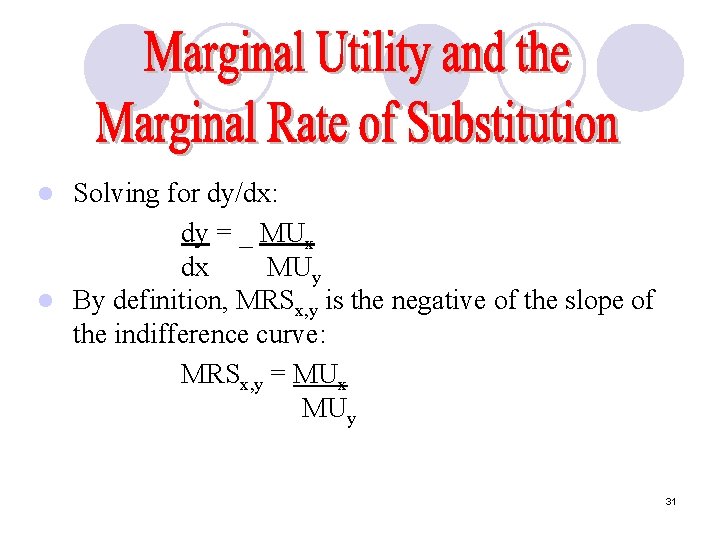
We can express the MRS for any basket as a ratio of the marginal utilities of the goods in that basket Suppose the consumer changes the level of consumption of x and y. Using differentials: d. U = MUx. dx + MUy. dy l Along a particular indifference curve, d. U = 0, so: 0 = MUx. dx + MUy. dy l 30

Solving for dy/dx: dy = _ MUx dx MUy l By definition, MRSx, y is the negative of the slope of the indifference curve: MRSx, y = MUx MUy l 31

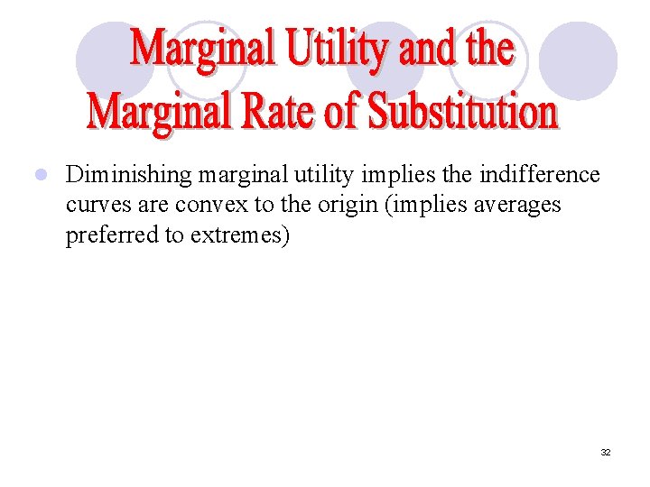
l Diminishing marginal utility implies the indifference curves are convex to the origin (implies averages preferred to extremes) 32

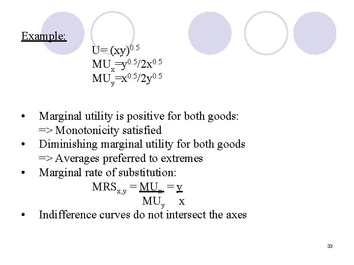
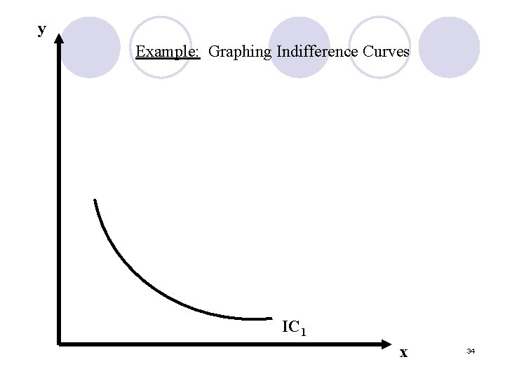
Example: U= (xy)0. 5 MUx=y 0. 5/2 x 0. 5 MUy=x 0. 5/2 y 0. 5 • • Marginal utility is positive for both goods: => Monotonicity satisfied Diminishing marginal utility for both goods => Averages preferred to extremes Marginal rate of substitution: MRSx, y = MUx = y MUy x Indifference curves do not intersect the axes 33

y Example: Graphing Indifference Curves IC 1 x 34

y Example: Graphing Indifference Curves Preference direction IC 2 IC 1 x 35

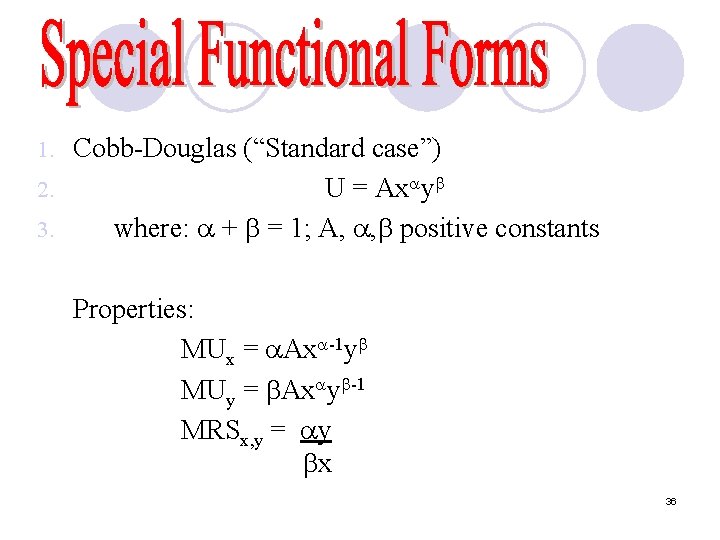
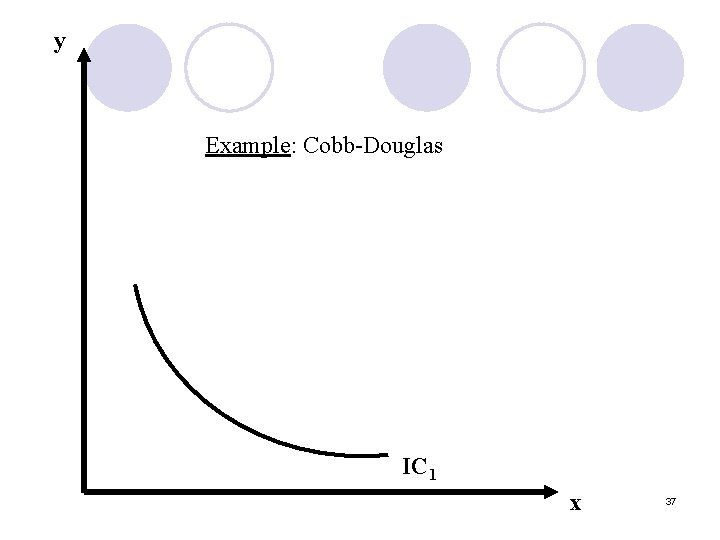
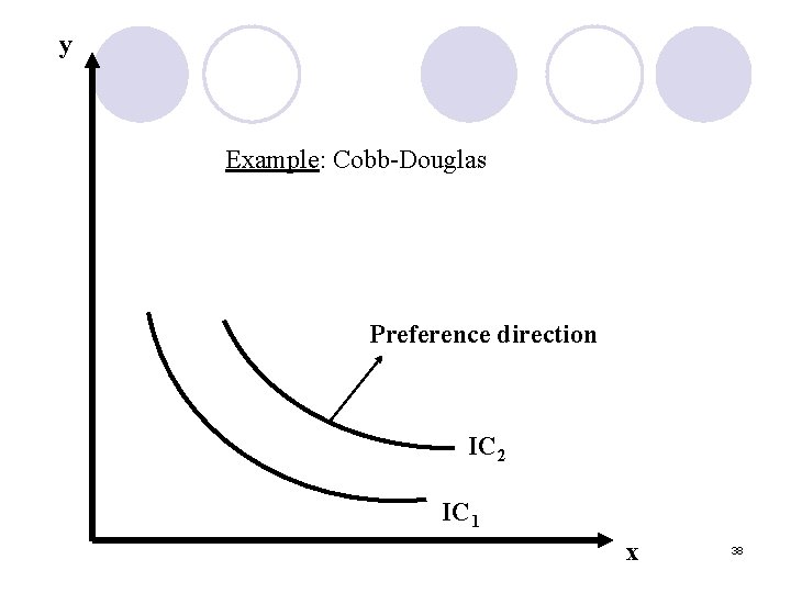
Cobb-Douglas (“Standard case”) 2. U = Ax y where: + = 1; A, , positive constants 3. 1. Properties: MUx = Ax -1 y MUy = Ax y -1 MRSx, y = y x 36

y Example: Cobb-Douglas IC 1 x 37

y Example: Cobb-Douglas Preference direction IC 2 IC 1 x 38

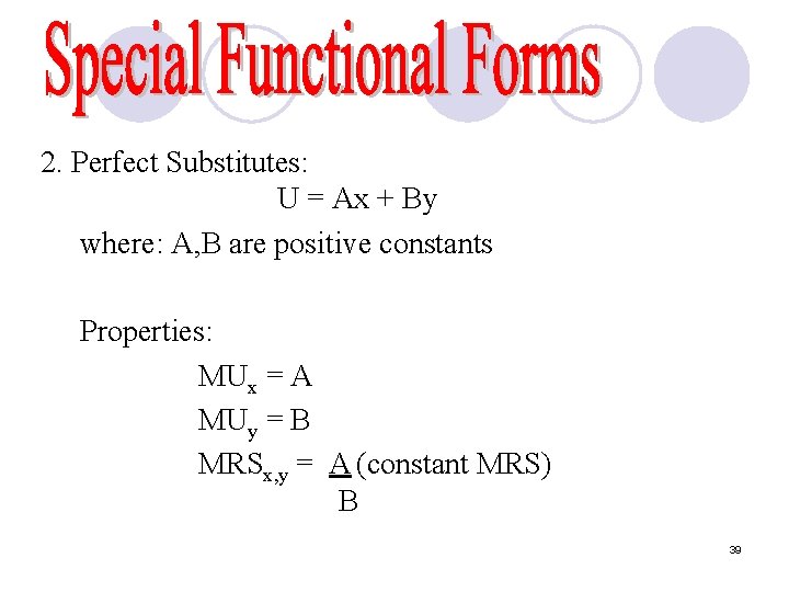
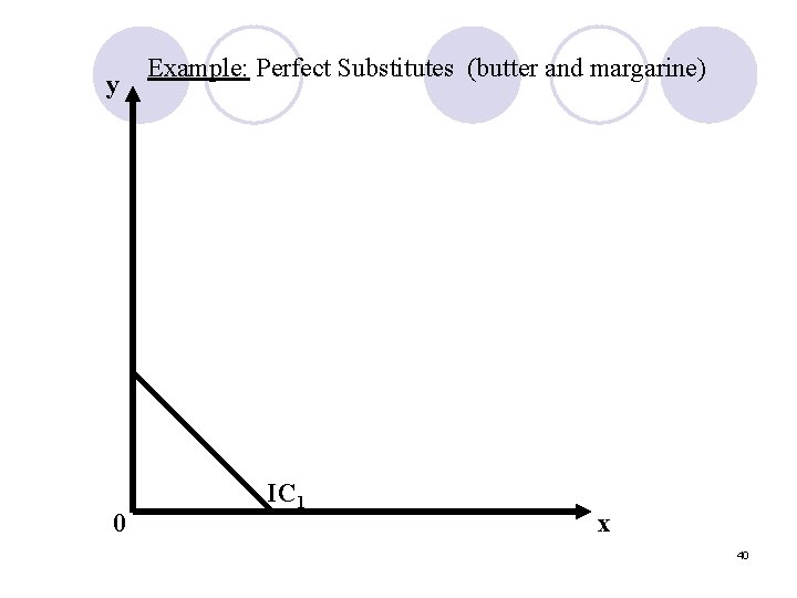
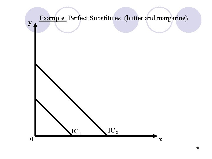
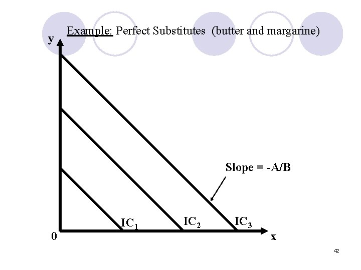
2. Perfect Substitutes: U = Ax + By where: A, B are positive constants Properties: MUx = A MUy = B MRSx, y = A (constant MRS) B 39

y 0 Example: Perfect Substitutes (butter and margarine) IC 1 x 40

y 0 Example: Perfect Substitutes (butter and margarine) IC 1 IC 2 x 41

y Example: Perfect Substitutes (butter and margarine) Slope = -A/B 0 IC 1 IC 2 IC 3 x 42

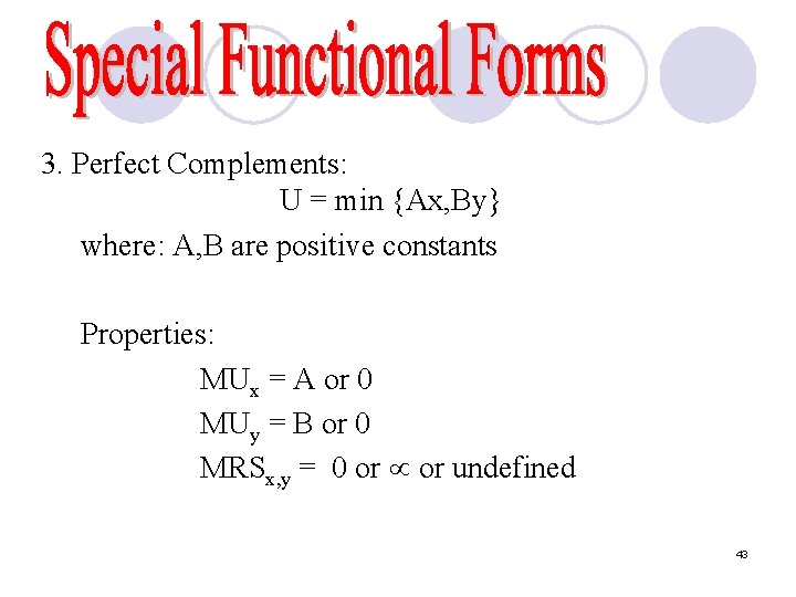
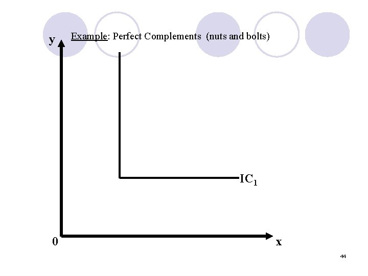
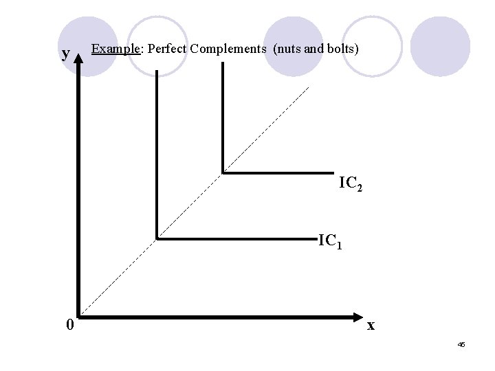
3. Perfect Complements: U = min {Ax, By} where: A, B are positive constants Properties: MUx = A or 0 MUy = B or 0 MRSx, y = 0 or undefined 43

y Example: Perfect Complements (nuts and bolts) IC 1 0 x 44

y Example: Perfect Complements (nuts and bolts) IC 2 IC 1 0 x 45

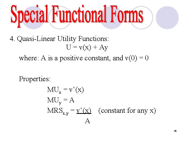
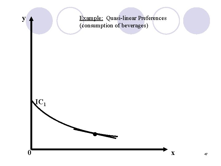
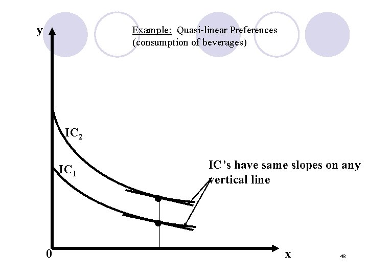
4. Quasi-Linear Utility Functions: U = v(x) + Ay where: A is a positive constant, and v(0) = 0 Properties: MUx = v’(x) MUy = A MRSx, y = v’(x) (constant for any x) A 46

y Example: Quasi-linear Preferences (consumption of beverages) IC 1 • 0 x 47

y Example: Quasi-linear Preferences (consumption of beverages) IC 2 IC 1 • • 0 IC’s have same slopes on any vertical line x 48

1. Characterization of consumer preferences without any restrictions imposed by budget 2. Minimal assumptions on preferences to get interesting conclusions on demand…seem to be satisfied for most people. (ordinal utility function) 49