Learning Mixtures of Arbitrary Distributions over Large Discrete

Learning Mixtures of Arbitrary Distributions over Large Discrete Domains Chaitanya Swamy University of Waterloo Leonard Schulman Yuval Rabani Caltech Hebrew University

Mixture learning problem Mixture source (w, P = {p 1, . . . , pk}) : • k arbitrary distributions over n items (n ≫ k): p 1, . . . pk ∈ Dn– 1 ≜ {x ∈ R+n– 1: ∑i xi = 1} • k mixture weights w 1, . . . , wk ≥ 0 s. t. ∑t wt = 1 Goal: Learn the mixture parameters given access to samples from the mixture source What kind of sampling access do we need/have? s-snapshot sample: choose pt with probability wt; pick s independent samples from pt to get a vector in [n]s

Mixture learning problem Goal: Learn the mixture parameters given access to s-snapshot samples (for some s) How does complexity of task vary with snapshot size s and number of samples? s=1: cannot learn anything more than the expected distribution ∑t wt pt ⇒ need s>1 Seek to keep sample size as low as possible, while minimizing dependence on snapshot size We call maximum snapshot size = aperture

Motivation • Natural, clean problem • Learning topic models from a corpus of documents. – Pure documents model: each document is a bag of words generated by sampling a topic + generating words according to the topic’s distribution. – So items º words, topics º mixture constituents, document º multi-snapshot sample. (Note n = vocabulary ≫ k = no. of topics; want to be able to work with small

Previous work Anandkumar-Hsu-Kakade (AHK), Anandkumar et al. (A+), Arora-Ge-Moitra (AGM): If p 1, . . . , pk are linearly independent (or satisfy an even stronger condition), then using • constant aperture (3 or 4) • poly(k, n) = W(n 3/e 2) sample size can reconstruct mixture constituents within l 1 -error e. (Some of this work also applies to the non-pure setting, where a document is generated by a topic-mixture using a mixture-distribution that also needs to be learnt. ) Status of the problem with arbitrary distributions was open.

Our work • Obtain the first bounds for arbitrary mixtures. We use O(n. polylog(n). poly(k/e)) + O(k/e)O(k 2) samples (2 k-1)-snapshots 1 -, 2 snapshots efficiently the mixture weights and reconstruct constitutents within l 1 -error e. • This is optimal aperture and near-optimal dependence on n. – Need W(n/e 2) samples to learn even a single distribution over [n] (or expectation of mixture) within l 1 -error e – Aperture 2 k-1 is the smallest aperture at which recovery is information-theoretically possible (to arbitrary accuracy) – Exponential dependence on k is necessary with aperture O(k) or even O(k. log n) (even for transportation-distance-e

Our work • Obtain the first bounds for arbitrary mixtures. We use O(n. polylog(n). poly(k/e)) + O(k/e)O(k 2) samples and reconstruct efficiently the mixture weights and constitutents within l 1 -error e. • This is optimal aperture and near-optimal dependence on n. • Concrete evidence that arbitrary mixtures are harder: – O(1) aperture, poly(k) sample size impossible for arbitrary mixtures • Key distinctions and challenges compared to previous work: – control error rate with O(n. polylog(n)) samples – quite noisy (with W(n 3) samples, challenge is to reconstruct from this relatively noiseless data on 3 -snapshots) – Need to deal with one-dimensional case (affine hull of P is a

The Algorithm Recall P = {p 1, . . . , pk}. Let r = ∑t wt pt , r). d=rank(p 1 -r, . . . , pk- Suffices to consider isotropic mixtures: ri is Q(1/n). Can split/delete items to move to an isotropic mixture (and aggregate items to move back), so focus on learning isotropic mixtures in the sequel.

Algorithm for isotropic mixtures Recall P = {p 1, . . . , pk}. Let r = ∑t wt pt , d=rank(p 1 -r, . . . , pkr). 1) Reduce dimension to d by learning aff(P), the affine hull of P. – Estimate r (easy). – Use spectral techniques to learn aff(P) from 2 -snapshots. Challenge: show that covariance matrix A = ∑t wt (pt – r)T can be approximated well using O(n. polylog(n)) samples.

Algorithm for isotropic mixtures Recall P = {p 1, . . . , pk}. Let r = ∑t wt pt , d=rank(p 1 -r, . . . , pkr). 1) Reduce dimension to d by learning aff(P), the affine hull of P. 2) Reduce to one-dimensional (1 D) case. – Pick a random orthonormal basis {b 1, . . . , bd} of inferred aff(P). – Project mixture (i. e. , snapshots) to each vector bj by mapping item i to bji – gives a 1 D distribution with support {bj 1, . . . , bjn}. – Challenge: show that if p, q ∈ P have large variation distance, then their projections b. Tp, b. Tq are also far apart relative to the support {b 1, . . . , bn} of projected distribution.

Algorithm for isotropic mixtures Recall P = {p 1, . . . , pk}. Let r = ∑t wt pt , d=rank(p 1 -r, . . . , pkr). 1) Reduce dimension to d by learning aff(P), the affine hull of P. 2) Reduce to one-dimensional (1 D) case. – Pick a random orthonormal basis {b 1, . . . , bd} of inferred aff(P). – Project mixture (i. e. , snapshots) to each vector bj by mapping item i to bji – gives a 1 D distribution with support {bj 1, . . . , bjn}. – For each bj, learn the k-spike 1 D mixture that assigns weight wt to the point (bj)Tpt = (expected value of projected mixture).

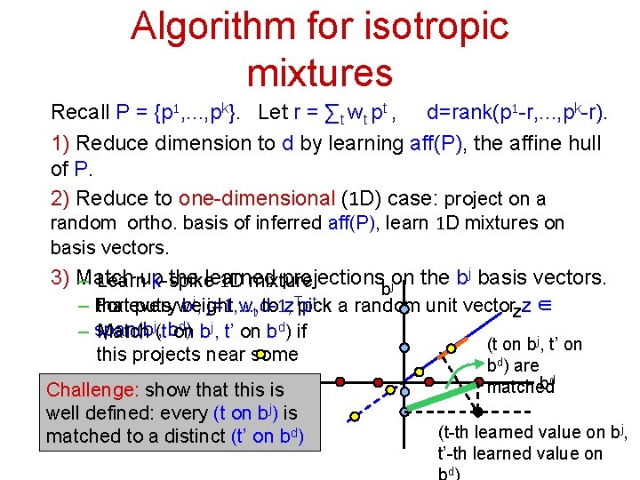
Algorithm for isotropic mixtures Recall P = {p 1, . . . , pk}. Let r = ∑t wt pt , d=rank(p 1 -r, . . . , pk-r). 1) Reduce dimension to d by learning aff(P), the affine hull of P. 2) Reduce to one-dimensional (1 D) case: project on a random ortho. basis of inferred aff(P), learn 1 D mixtures on basis vectors. 3) Match the learned projections on the bj basis vectors. – Learnup k-spike 1 D mixture j b thatevery puts weight wt to z. Tpick pt a random unit vectorzz ∈ – For bj, j=1, . . . , d-1, d) j , bon – span(b Match j(t b , t’ on bd) if (t on bj, t’ on this projects near some bd) are on z bd matched Challenge: show that this is well defined: every (t on bj) is (t-th learned value on bj, matched to a distinct (t’ on bd) t’-th learned value on d

Algorithm for isotropic mixtures Recall P = {p 1, . . . , pk}. Let r = ∑t wt pt , d=rank(p 1 -r, . . . , pkr). 1) Reduce dimension to d by learning aff(P), the affine hull of P. 2) Reduce to one-dimensional (1 D) case: project on a random ortho. basis of inferred aff(P), learn 1 D mixtures on basis vectors. 3) Match up the learned projections on the bj basis vectors. 4) Use estimate r’ of r, and the matched-up learned projections to compute a point qt in r’ + span(b 1, . . . , bd), and weight w’t for each pt. Project the qt’s to Dn– 1 to obtain the learnt mixture.

Algorithm for isotropic mixtures Recall P = {p 1, . . . , pk}. Let r = ∑t wt pt , d=rank(p 1 -r, . . . , pkr). 1) Reduce dimension to d by learning aff(P), the affine hull of P. 2) Reduce to one-dimensional (1 D) case. – Pick a random orthonormal basis {b 1, . . . , bd} of inferred aff(P). – Project mixture (i. e. , snapshots) to each vector bj by mapping item i to bji – gives a 1 D distribution with support {bj 1, . . . , bjn}. – For each bj, learn the k-spike 1 D mixture that assigns weight wt to the point (bj)T pt = (expected value of projected mixture).

1 D mixture-learning problem Let b: given basis vector. Input: mixture placing weight wt to distribution with support {b 1, . . . , bn} and expectation b. Tpt derived from projecting pt on b Goal: Learn the wt’s and the expectations {b. Tp 1, . . . , b. Tpk} By scaling and translation, we may assume that each 1 D source is supported on [0, 1] Important: scaling does not much affect separation between sources: 1/√n-factor arising due to l 1→ l 2 conversion is canceled by 1/√n l¥-norm bound on b

1 D mixture-learning problem Let b: given basis vector. Input: mixture placing weight wt to distribution with support {b 1, . . . , bn} and expectation b. Tpt derived from projecting pt on b Goal: Learn the wt’s and the expectations {b. Tp 1, . . . , b. Tpk} Use randomized-rounding trick to reduce to learning a mixture of “coins” Coin-learning problem input: bag of k coins; coin t occurs with probability wt and has bias b. Tpt Goal: Learn the mixture weights and biases Aperture 2 k-1, i. e. , 2 k-1 throws of a sampled coin, is necessary.

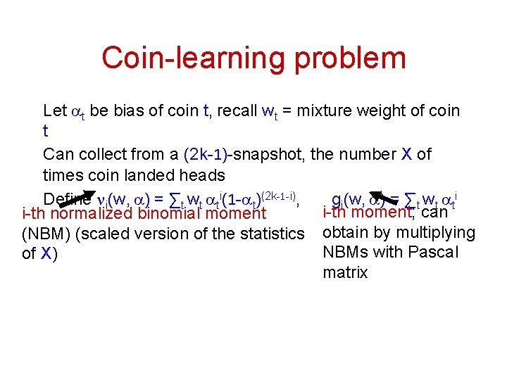
Coin-learning problem Let at be bias of coin t, recall wt = mixture weight of coin t Can collect from a (2 k-1)-snapshot, the number X of times coin landed heads Define ni(w, a) = ∑t wt ati(1 -at)(2 k-1 -i), gi(w, a) = ∑t wt ati i-th moment; can i-th normalized binomial moment (NBM) (scaled version of the statistics obtain by multiplying NBMs with Pascal of X) matrix

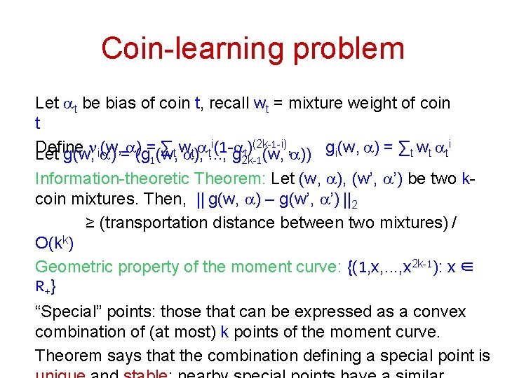
Coin-learning problem Let at be bias of coin t, recall wt = mixture weight of coin t i(1 -a )(2 k-1 -i), i Define n (w, a) = ∑ w a g (w, a) = ∑ w a i t t t Let g(w, a) = (g (w, a), . . . , g (w, a)) 1 2 k-1 Information-theoretic Theorem: Let (w, a), (w’, a’) be two kcoin mixtures. Then, || g(w, a) – g(w’, a’) ||2 ≥ (transportation distance between two mixtures) / O(kk) Geometric property of the moment curve: {(1, x, . . . , x 2 k-1): x ∈ R+} “Special” points: those that can be expressed as a convex combination of (at most) k points of the moment curve. Theorem says that the combination defining a special point is

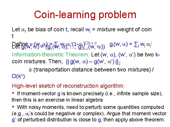
Coin-learning problem Let at be bias of coin t, recall wt = mixture weight of coin t i(1 -a )(2 k-1 -i), i Define n (w, a) = ∑ w a g (w, a) = ∑ w a t t. . . , g t (w, a)) i t t t Let g(w, ia) = (g (w, t a), 1 2 k-1 Information-theoretic Theorem: Let (w, a), (w’, a’) be two kcoin mixtures. Then, || g(w, a) – g(w’, a’) ||2 ≥ (transportation distance between two mixtures) / O(kk) High-level sketch of reconstruction algorithm: • If moment-vector g is known precisely (i. e. , infinte sample size), then this is an exercise in linear algebra • With noisy moments, need to perturb some quantities computed (e. g. , at’s could be negative or complex). Argue that moment vector g’ of perturbed distribution is close to g, then apply above theorem.

Thank You