Learning Microsoft Excel 2007 Getting Started There are

Learning Microsoft Excel 2007

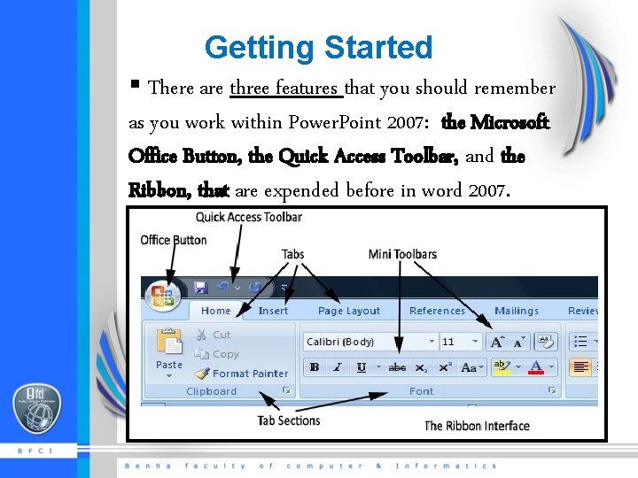
Getting Started § There are three features that you should remember as you work within Power. Point 2007: the Microsoft Office Button, the Quick Access Toolbar, and the Ribbon, that are expended before in word 2007.

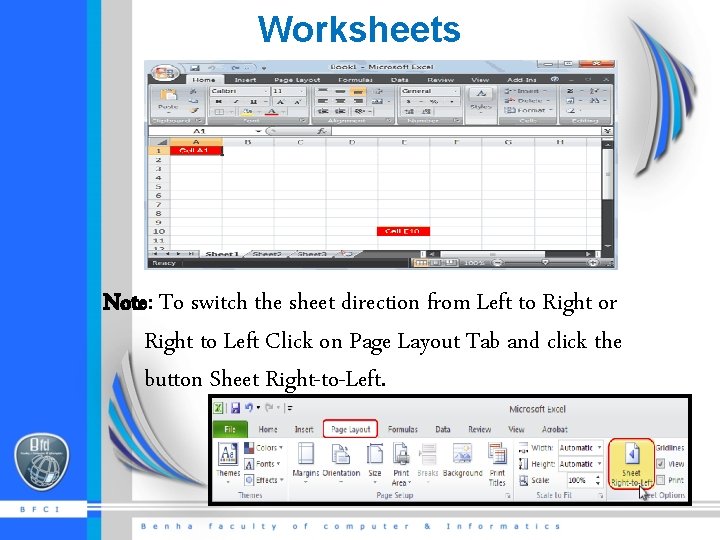
Worksheets Note: To switch the sheet direction from Left to Right or Right to Left Click on Page Layout Tab and click the button Sheet Right-to-Left.

Worksheets (Conts) 1. Microsoft Excel consists of worksheets. Each worksheet contains columns and rows. 2. A cell is where the column and row intersect. 3. For example, the cell located in the upper-left corner of the worksheet is cell A 1, meaning column A, row 1. and cell E 10 is located under column E on row 10. You enter your data into the cells on the worksheet. 4. Groups of cells are called ranges or blocks; can be selected with mouse or keyboard

Move around a Worksheet § By using the arrow keys, you can move around your selected worksheet. § You can use the down arrow key to move downward one cell at a time. § You can use the up arrow key to move upward one cell at a time. § You can use the right and left arrow keys to move right or left one cell at a time. § The Page Up and Page Down keys move up and down one page at a time.

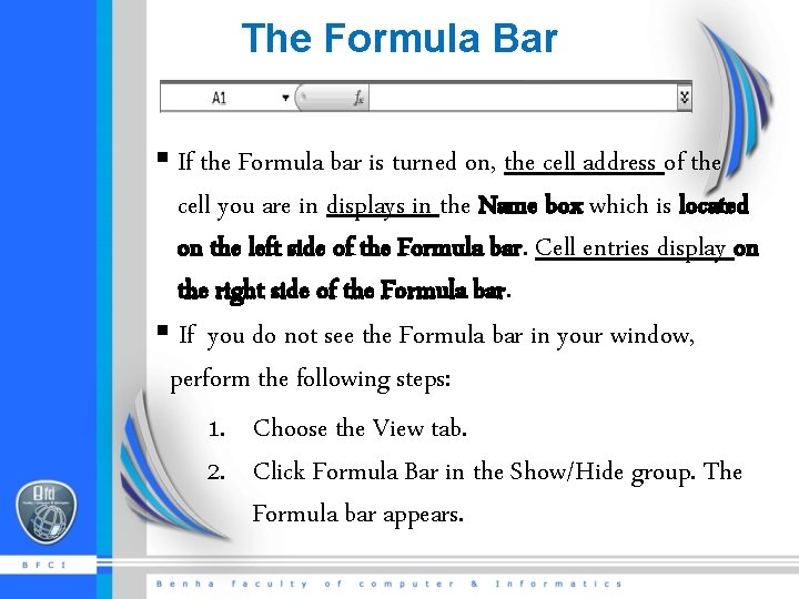
The Formula Bar § If the Formula bar is turned on, the cell address of the cell you are in displays in the Name box which is located on the left side of the Formula bar. Cell entries display on the right side of the Formula bar. § If you do not see the Formula bar in your window, perform the following steps: 1. Choose the View tab. 2. Click Formula Bar in the Show/Hide group. The Formula bar appears.

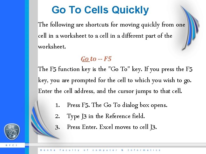
Go To Cells Quickly The following are shortcuts for moving quickly from one cell in a worksheet to a cell in a different part of the worksheet. Go to -- F 5 The F 5 function key is the "Go To" key. If you press the F 5 key, you are prompted for the cell to which you wish to go. Enter the cell address, and the cursor jumps to that cell. 1. Press F 5. The Go To dialog box opens. 2. Type J 3 in the Reference field. 3. Press Enter. Excel moves to cell J 3.

Go To Cells Quickly (Conts) Go to -- Ctrl+G You can also use Ctrl+G to go to a specific cell. 1. Hold down the Ctrl key while you press "g" (Ctrl+g). The Go To dialog box opens. 2. Type C 4 in the Reference field. 3. Press Enter. Excel moves to cell C 4.

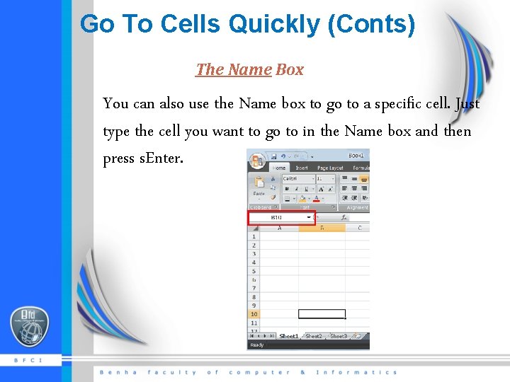
Go To Cells Quickly (Conts) The Name Box You can also use the Name box to go to a specific cell. Just type the cell you want to go to in the Name box and then press s. Enter.

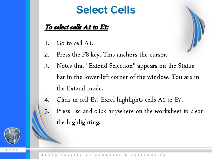
Select Cells To select cells A 1 to E 1: 1. Go to cell A 1. 2. Press the F 8 key. This anchors the cursor. 3. Notes that "Extend Selection" appears on the Status bar in the lower-left corner of the window. You are in the Extend mode. 4. Click in cell E 7. Excel highlights cells A 1 to E 7. 5. Press Esc and click anywhere on the worksheet to clear the highlighting.

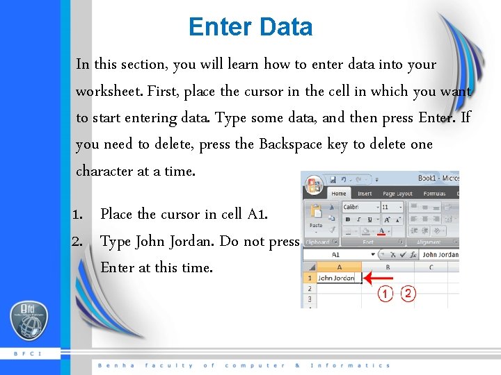
Enter Data In this section, you will learn how to enter data into your worksheet. First, place the cursor in the cell in which you want to start entering data. Type some data, and then press Enter. If you need to delete, press the Backspace key to delete one character at a time. 1. Place the cursor in cell A 1. 2. Type John Jordan. Do not press Enter at this time.

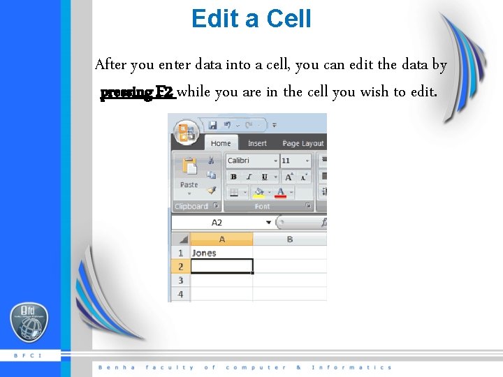
Edit a Cell After you enter data into a cell, you can edit the data by pressing F 2 while you are in the cell you wish to edit.

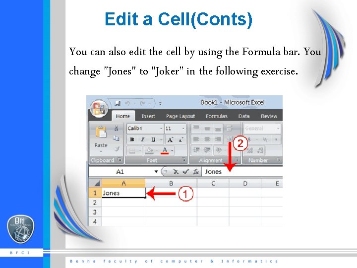
Edit a Cell(Conts) You can also edit the cell by using the Formula bar. You change "Jones" to "Joker" in the following exercise.

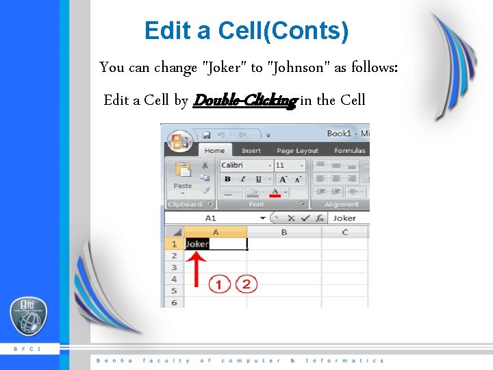
Edit a Cell(Conts) You can change "Joker" to "Johnson" as follows: Edit a Cell by Double-Clicking in the Cell

Change a Cell Entry Typing in a cell replaces the old cell entry with the new information you type.

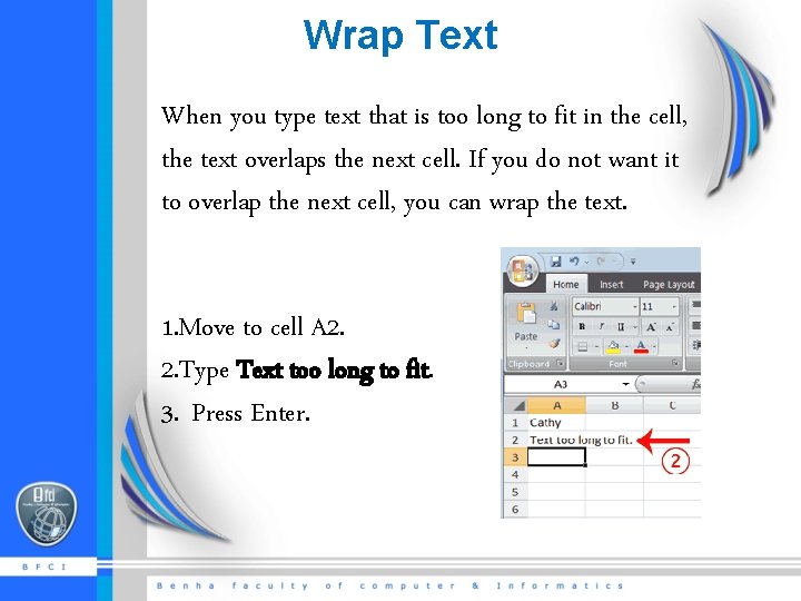
Wrap Text When you type text that is too long to fit in the cell, the text overlaps the next cell. If you do not want it to overlap the next cell, you can wrap the text. 1. Move to cell A 2. 2. Type Text too long to fit. 3. Press Enter.

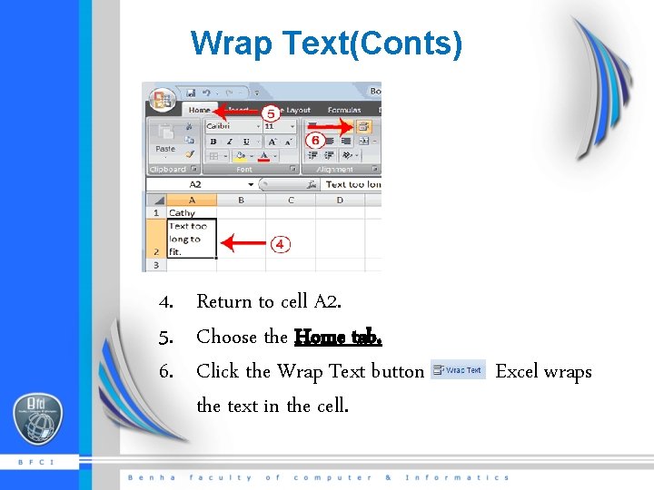
Wrap Text(Conts) 4. Return to cell A 2. 5. Choose the Home tab. 6. Click the Wrap Text button the text in the cell. Excel wraps

Delete a Cell Entry To delete an entry in a cell or a group of cells, you place the cursor in the cell or select the group of cells and press Delete. 1. Select cells A 1 to A 2. 2. Press the Delete key.

Entering Excel Formulas

Perform Mathematical Calculations In Microsoft Excel, you can enter numbers and mathematical formulas into cells. Whether you enter a number or a formula, you can reference the cell when you perform mathematical calculations such as addition, subtraction, multiplication, or division. When entering a mathematical formula, precede the formula with an equal sign. Use the following to indicate the type of calculation you wish to perform: + Addition / Division - Subtraction ^ Exponential * Multiplication

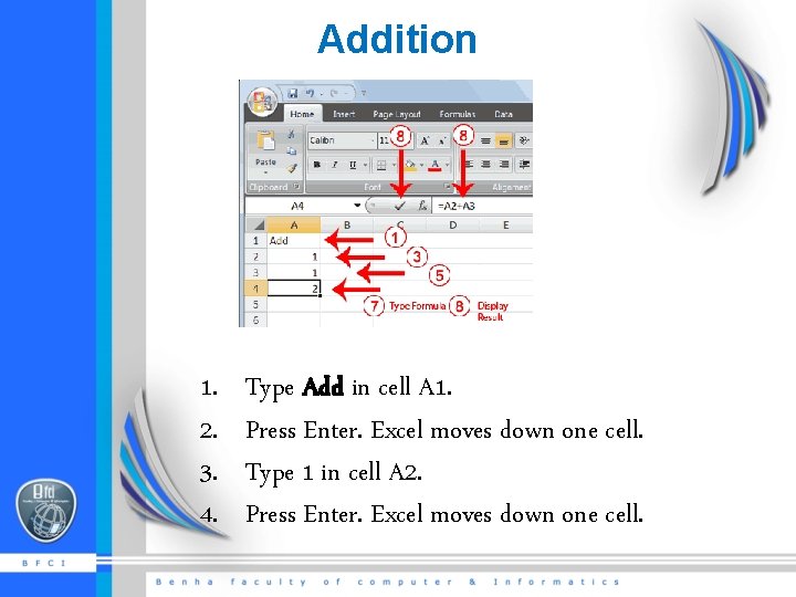
Addition 1. 2. 3. 4. Type Add in cell A 1. Press Enter. Excel moves down one cell. Type 1 in cell A 2. Press Enter. Excel moves down one cell.

Addition(Conts) 5. 6. 7. 8. Type 1 in cell A 3. Press Enter. Excel moves down one cell. Type =A 2+A 3 in cell A 4. Click the check mark on the Formula bar. Excel adds cell A 1 to cell A 2 and displays the result in cell A 4. The formula displays on the Formula bar. Note: Clicking the check mark on the Formula bar is similar to pressing Enter. Excel records your entry but does not move to the next cell.

Auto. Sum § You can use the Auto. Sum button on the Home tab to automatically add a column or row of numbers. § When you press the Auto. Sum button , Excel selects the numbers it thinks you want to add. If you then click the check mark on the Formula bar or press the Enter key, Excel adds the numbers. § If Excel's guess as to which numbers you want to add is wrong, you can select the cells you want.

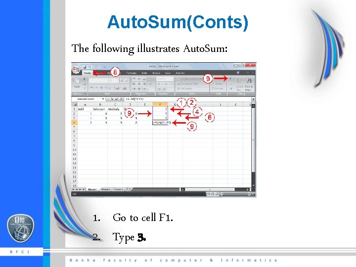
Auto. Sum(Conts) The following illustrates Auto. Sum: 1. Go to cell F 1. 2. Type 3.

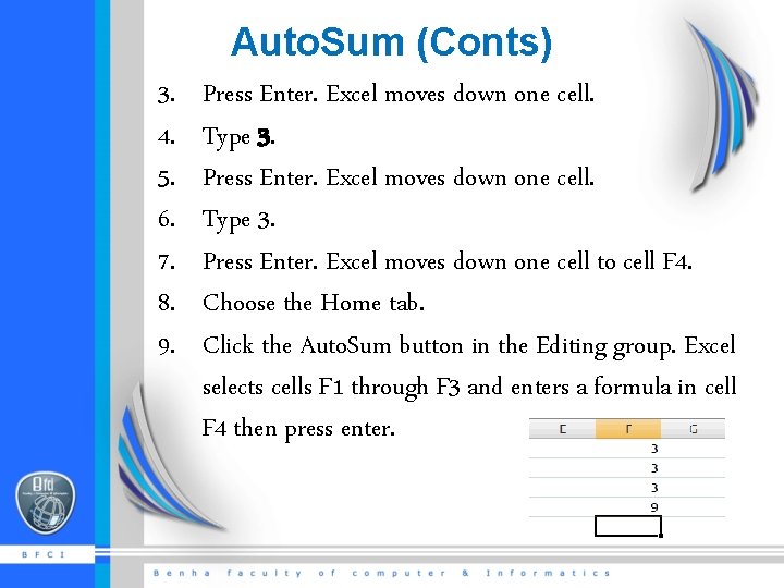
Auto. Sum (Conts) 3. 4. 5. 6. 7. 8. 9. Press Enter. Excel moves down one cell. Type 3. Press Enter. Excel moves down one cell to cell F 4. Choose the Home tab. Click the Auto. Sum button in the Editing group. Excel selects cells F 1 through F 3 and enters a formula in cell F 4 then press enter.

Perform Automatic Calculations By default, Microsoft Excel recalculates the worksheet as you change cell entries. This makes it easy for you to correct mistakes and analyze a variety of scenarios.

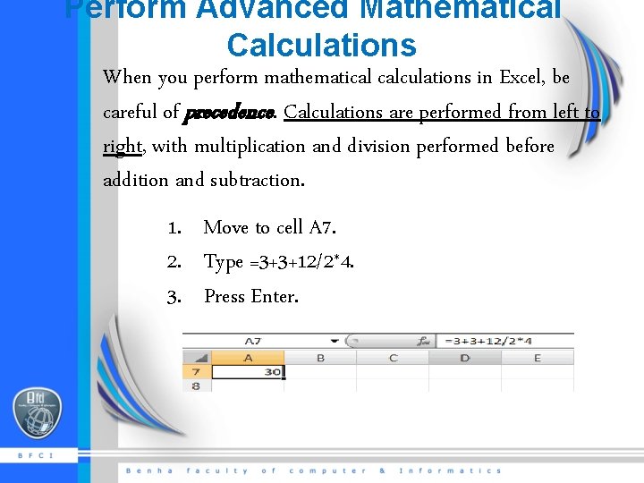
Perform Advanced Mathematical Calculations When you perform mathematical calculations in Excel, be careful of precedence. Calculations are performed from left to right, with multiplication and division performed before addition and subtraction. 1. Move to cell A 7. 2. Type =3+3+12/2*4. 3. Press Enter.

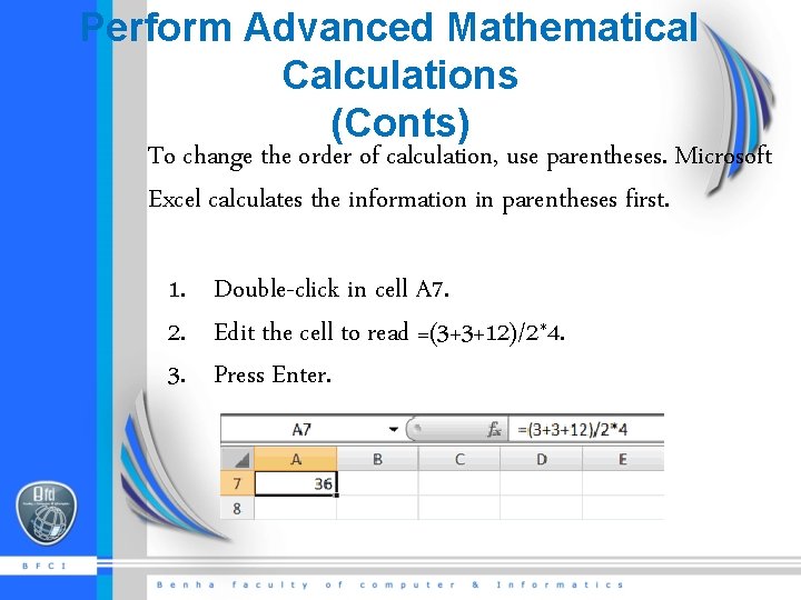
Perform Advanced Mathematical Calculations (Conts) To change the order of calculation, use parentheses. Microsoft Excel calculates the information in parentheses first. 1. Double-click in cell A 7. 2. Edit the cell to read =(3+3+12)/2*4. 3. Press Enter.

Formatting Data

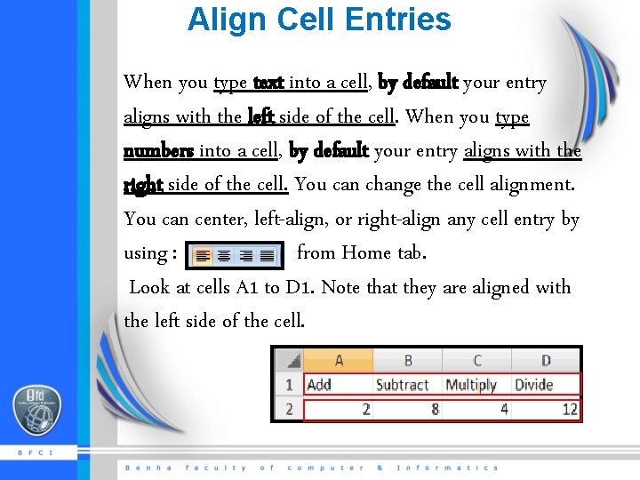
Align Cell Entries When you type text into a cell, by default your entry aligns with the left side of the cell. When you type numbers into a cell, by default your entry aligns with the right side of the cell. You can change the cell alignment. You can center, left-align, or right-align any cell entry by using : from Home tab. Look at cells A 1 to D 1. Note that they are aligned with the left side of the cell.

Copy, Cut, Paste, and Cell Addressing § In Excel, you can copy data from one area of a worksheet and place the data you copied anywhere in the same or another worksheet. Simple copy it and then paste it in the new location. § You can use Excel's Cut feature to remove information from a worksheet. Then you can use the Paste feature to place the information you cut anywhere in the same or another worksheet.

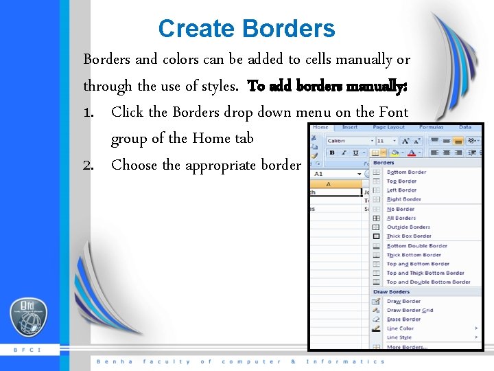
Create Borders and colors can be added to cells manually or through the use of styles. To add borders manually: 1. Click the Borders drop down menu on the Font group of the Home tab 2. Choose the appropriate border

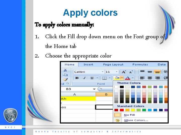
Apply colors To apply colors manually: 1. Click the Fill drop down menu on the Font group of the Home tab 2. Choose the appropriate color

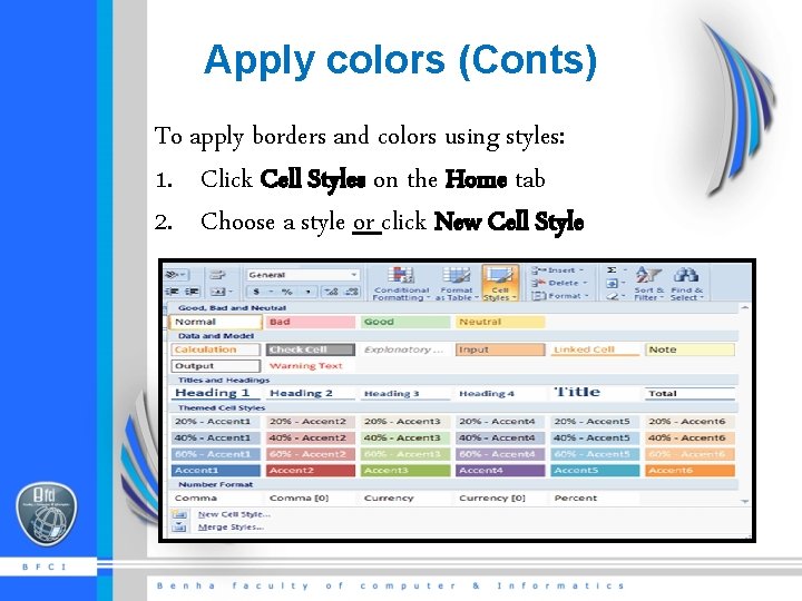
Apply colors (Conts) To apply borders and colors using styles: 1. Click Cell Styles on the Home tab 2. Choose a style or click New Cell Style

Format Numbers

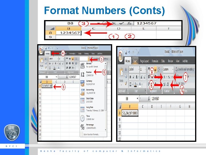
Format Numbers Format the numbers that entered into Microsoft Excel. For example, you can add commas to separate thousands, specify the number of decimal places, place a dollar sign in front of a number, or display a number as a percent. 1. The Method for Formatting numbers (Example): 1. Move to cell B 8. 2. Type 1234567. 3. Click the check mark on the Formula bar. 4. Choose the Home tab. 5. Click the down arrow next to the Number Format box A menu appears.

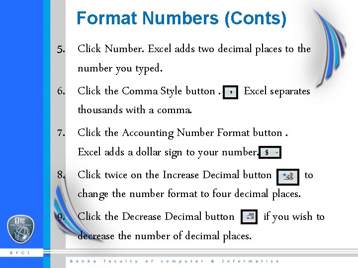
Format Numbers (Conts) 5. Click Number. Excel adds two decimal places to the number you typed. 6. Click the Comma Style button. Excel separates thousands with a comma. 7. Click the Accounting Number Format button. Excel adds a dollar sign to your number. 8. Click twice on the Increase Decimal button to change the number format to four decimal places. 9. Click the Decrease Decimal button if you wish to decrease the number of decimal places.

Format Numbers (Conts)

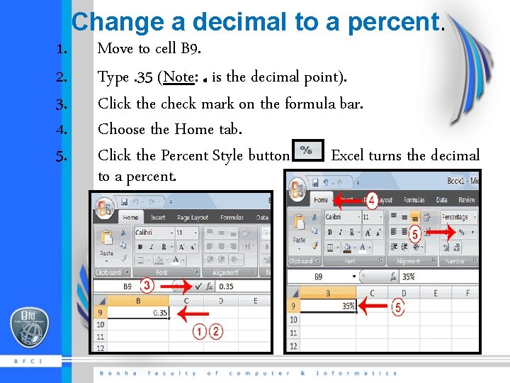
Change a decimal to a percent. 1. 2. 3. 4. 5. Move to cell B 9. Type. 35 (Note: . is the decimal point). Click the check mark on the formula bar. Choose the Home tab. Click the Percent Style button. Excel turns the decimal to a percent.

Creating Excel Functions, Filling Cells

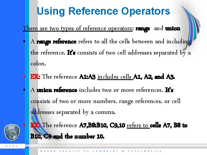
Using Reference Operators There are two types of reference operators: range and union • A range reference refers to all the cells between and including the reference. It’s consists of two cell addresses separated by a colon. • EX: The reference A 1: A 3 includes cells A 1, A 2, and A 3. • A union reference includes two or more references. It’s consists of two or more numbers, range references, or cell addresses separated by a comma. • EX: The reference A 7, B 8: B 10, C 9, 10 refers to cells A 7, B 8 to B 10, C 9 and the number 10.

Understanding Functions

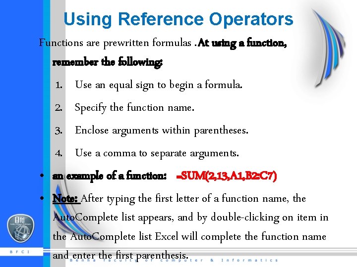
Using Reference Operators Functions are prewritten formulas. At using a function, remember the following: 1. Use an equal sign to begin a formula. 2. Specify the function name. 3. Enclose arguments within parentheses. 4. Use a comma to separate arguments. • an example of a function: =SUM(2, 13, A 1, B 2: C 7) • Note: After typing the first letter of a function name, the Auto. Complete list appears, and by double-clicking on item in the Auto. Complete list Excel will complete the function name and enter the first parenthesis.

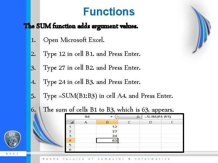
Functions The SUM function adds argument values. 1. Open Microsoft Excel. 2. Type 12 in cell B 1. and Press Enter. 3. Type 27 in cell B 2. and Press Enter. 4. Type 24 in cell B 3. and Press Enter. 5. Type =SUM(B 1: B 3) in cell A 4. and Press Enter. 6. The sum of cells B 1 to B 3, which is 63, appears.

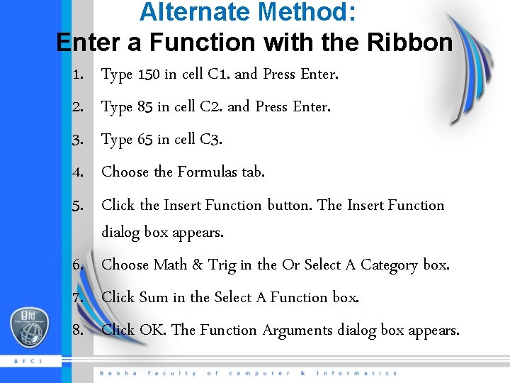
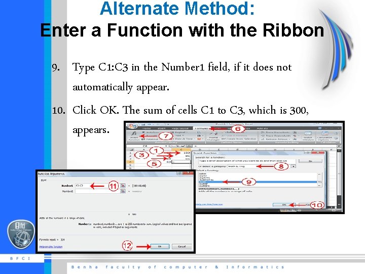
Alternate Method: Enter a Function with the Ribbon 1. 2. 3. 4. 5. Type 150 in cell C 1. and Press Enter. Type 85 in cell C 2. and Press Enter. Type 65 in cell C 3. Choose the Formulas tab. Click the Insert Function button. The Insert Function dialog box appears. 6. Choose Math & Trig in the Or Select A Category box. 7. Click Sum in the Select A Function box. 8. Click OK. The Function Arguments dialog box appears.

Alternate Method: Enter a Function with the Ribbon 9. Type C 1: C 3 in the Number 1 field, if it does not automatically appear. 10. Click OK. The sum of cells C 1 to C 3, which is 300, appears.

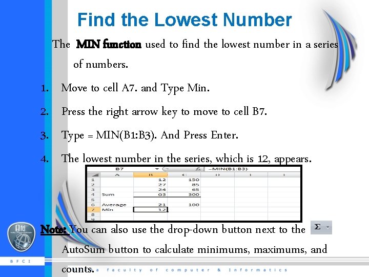
Find the Lowest Number The MIN function used to find the lowest number in a series of numbers. 1. Move to cell A 7. and Type Min. 2. Press the right arrow key to move to cell B 7. 3. Type = MIN(B 1: B 3). And Press Enter. 4. The lowest number in the series, which is 12, appears. Note: You can also use the drop-down button next to the Auto. Sum button to calculate minimums, maximums, and counts.

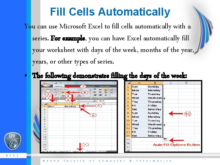
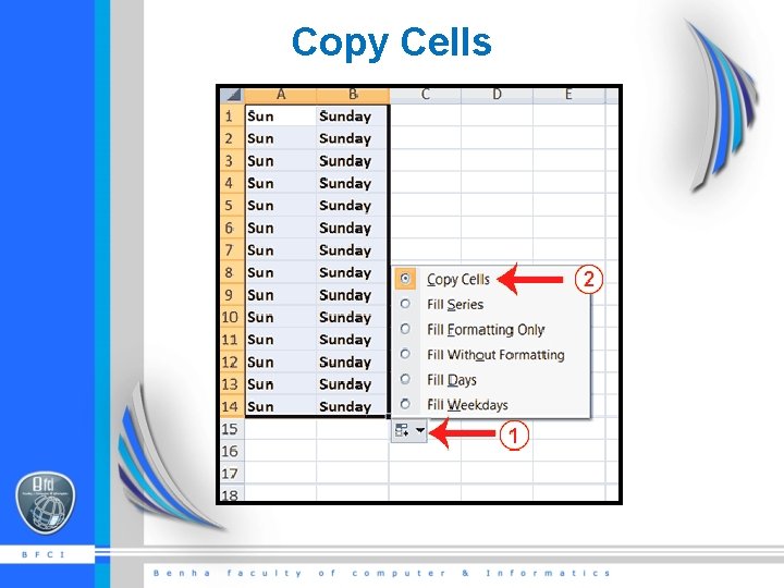
Fill Cells Automatically You can use Microsoft Excel to fill cells automatically with a series. For example, you can have Excel automatically fill your worksheet with days of the week, months of the year, years, or other types of series. • The following demonstrates filling the days of the week:

Copy Cells

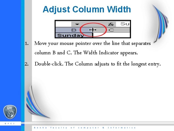
Adjust Column Width 1. Move your mouse pointer over the line that separates column B and C. The Width Indicator appears. 2. Double-click. The Column adjusts to fit the longest entry.

Fill Times & Fill Numbers • Type a data(numbers or times) in specific cell. • Grab the fill handle and drag with your mouse to highlight beginning cell to ending cell. The data fills each cell.

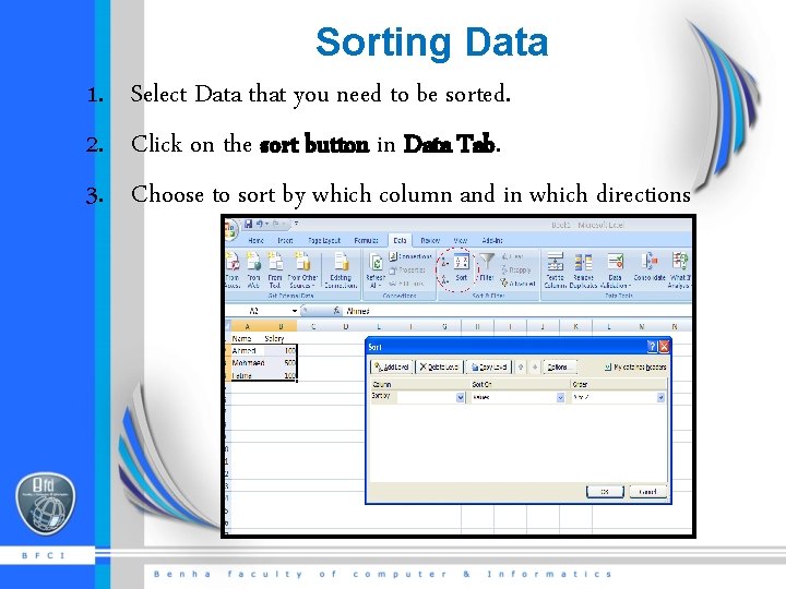
Sorting Data 1. Select Data that you need to be sorted. 2. Click on the sort button in Data Tab. 3. Choose to sort by which column and in which directions

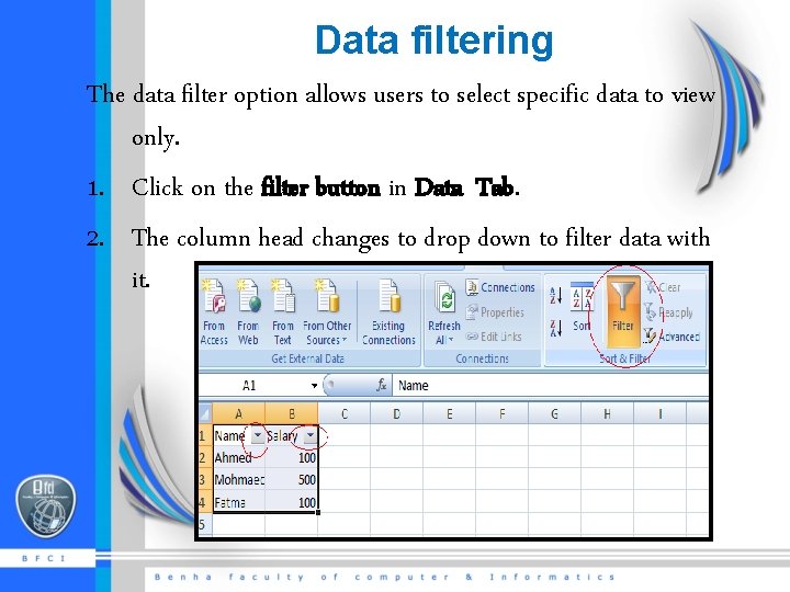
Data filtering The data filter option allows users to select specific data to view only. 1. Click on the filter button in Data Tab. 2. The column head changes to drop down to filter data with it.

Creating Charts Microsoft Excel, can represent numbers in a chart.

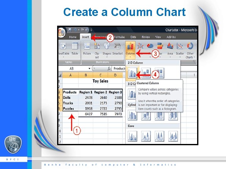
Create a Column Chart

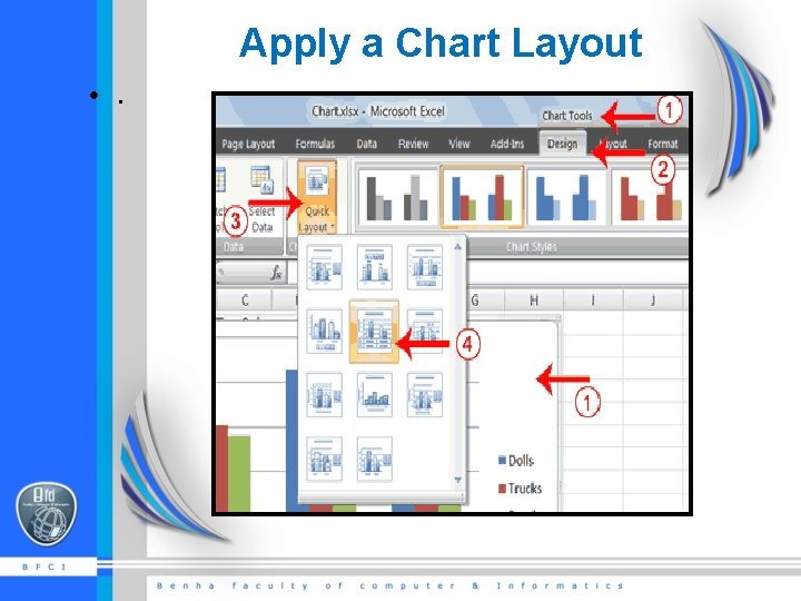
Apply a Chart Layout • .

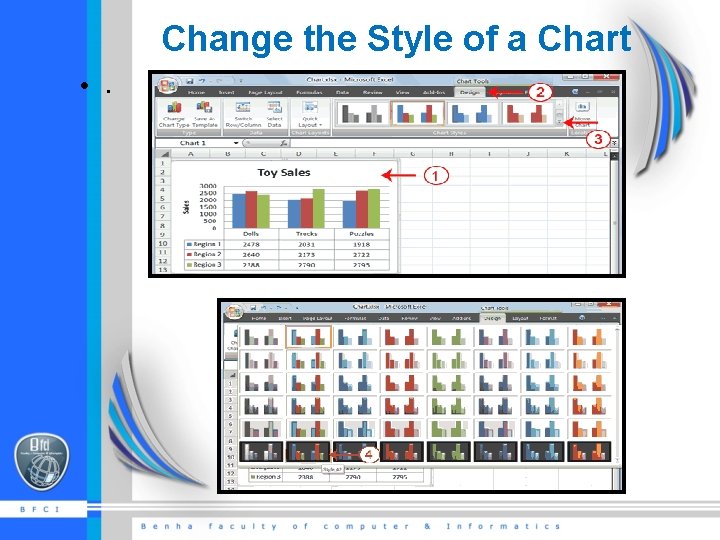
Change the Style of a Chart • .

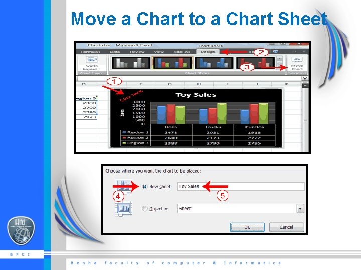
Move a Chart to a Chart Sheet

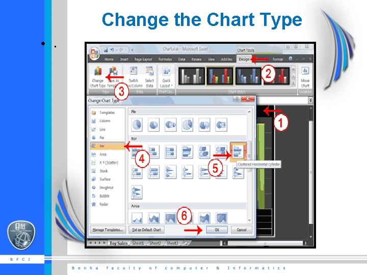
Change the Chart Type • .

The References • http: //www. baycongroup. com/el 0. htm • http: //www. exceldigest. com/myblog/2009/04/08/excel-2007 user-interface-page-layout-tab/ • http: //www. fgcu. edu/support/office 2007/excel/index. asp