Learning Deep Energy Models Jiquan Ngiam Zhenghao Chen

Learning Deep Energy Models Jiquan Ngiam Zhenghao Chen Pang Wei Koh Andrew Y. Ng

Energy-Based Models (EBM) • Energy-based models associate a scalar energy to each configuration of the variables of the interest • Learning corresponds to modifying that energy function • Desirable configurations will have low energy

Energy-Based Models (EBM) • Energy-based models define a probability distribution through an energy function: • Lower energy corresponds to higher probability • Z is the normalizing factor, called the partition function

Energy-Based Models (EBM) • An energy-based model can be learnt by stochastic gradient descent on the empirical negative log-likelihood of the training data • The log-likelihood and loss function is similar to those of logistic regression

EBM with Hidden Units • For a data x, it has a observable part (still denoted x) and hidden part h • The free energy is defined as • Which allows us to write

EBM with Hidden Units • Given • We have

EBM with Hidden Units • The data negative log-likelihood gradient is • Hence the average log-likelihood gradient over the training set is • P hat is the training set empirical distribution and P is the model’s distribution • Expectation over model distribution is hard to compute, usually computed through sampling

Restricted Boltzmann Machine • The energy function of an RBM is defined as where W is represents the weights connecting hidden and visible units, b and c are the offsets of the visible and hidden layers

Restricted Boltzmann Machine • Sampling in an RBM can be carried out using Gibbs sampling on a Markov chain • Efficient learning algorithms were found to train it

Deep Belief Network (DBN) • A deep belief network is a graphical model with undirected connections at the top hidden layers and directed connections in the lower layers • Greedy layerwise training by stacking restricted Boltzmann machines, each of which models the posterior distribution of the previous layer • Computationally expensive to train all layers of the DBN jointly

Deep Boltzmann Machine (DBM) • DBMs have undirected connections between all layers of the network. • A similar layerwise training algorithm using RMBs is used to initialize the DBM and all layers are jointly trained thereafter • Both DBNs and DBMs have multiple stochastic hidden layers, which makes inference and learning difficult as computing the conditional posterior over the hidden units intractable • Inference and learning are more tractable in models with only a single stochastic hidden layer (an RBM)

Deep Energy Models (DEM) • A feedforward neural network that deterministically transforms the input • Models the output of the feedforward network with a layer of stochastic hidden units – The feedforward neural network extracts features from the input which are more easily modeled with a single stochastic layer • Since the hidden variable of the feedforward neural network is deterministic, this allows us to efficiently train all layers of the network jointly

Deep Energy Models • Comparison of DBN, DBM and DEM • Dotted arrow in DEM represent deterministic relationships

Deep Energy Models • Let gθ(v) denote the feedforward output of a neural network gθ • The undirected connection between gθ(v) and the set of binary stochastic hidden units h defines an energy function

Learning Deep Energy Models • Model is trained by maximizing the log-likelihood of a training set • The parameters of the feedforward network gθ, variance parameter σ, weights W and biases c • The derivative of the log-likelihood is given by • The first term represents an expectation of the partial derivative over the model distribution and the second an expectation over the data • The second term is straightforward, but the first term requires sampling

Learning Deep Energy Models • To sample from the model distribution, Hybrid Monte Carlo (HMC) is used • HMC draw samples from the model distribution by performing a physical simulation of an energyconserving system to generate proposal moves • The method of using the HMC sampler to estimate the gradient of the data log-likelihood is known as contrastive backpropagation

Greedy Layerwise Training • DBN: training an RBM to model the posteriors of the hidden units in the previous layer • DEM: training the next layer to optimize for the data likelihood, but freeze the parameters of the earlier layers • The learning objective of DEM is the data likelihood of the entire deep model

Folding Hidden Layers • After training a network with l layers, we can “fold” the top hidden layer into the model by letting • Stochastic hidden layer -> deterministic • A next layer can then be trained using as the feedforward network

Joint Training for Multiple Layers • Simply unfreezes the weights of the previous layers while optimizing for the same objective function • On DBN and DBMs, it requires sampling all the hidden layers of the network • DEM does not require sampling hidden layers of the network as it use deterministic hidden units • In practice, it turns out that mixing greedy layerwise steps together with joint training steps performed well

The Product of Student-t Model • Products of Experts (Po. E) models – A restricted class of EBM – Distribution is the normalized product of all the distributions represented by the individual “experts” • Product of Student-t Model

General Form of DEM • The free energy can be defined as: • The original deep energy models can be viewed as having • By allowing other functions, we can recover models such as the product of Student-t (Po. T) • Stacked Po. T (SPo. T) model: we parameterize the neural network gθ to have log(1+z^2) as the activation function

Experiments on Natural Images • DEM with sigmoidal units (sigmoid-DEM) and the SPo. T models • M 1 -M 2 -M 12 denote models trained with greedy layerwise on the 1 st, 2 nd layer respectively, followed by a joint training on the 1 st and 2 nd layer.

Experiments on Natural Images • The first layer M 1 quickly plateaus • Adding the second layer improves performance • Joint training resulted in a further improvement

Generative Deep Energy Models • The activations of each layer in gθ as features which are used to learn a linear classifier for some associated labels y, with weights U. • The joint energy between the inputs v and labels y is where al are the activation of the lth layer and y is a one-hot vector of image labels. • Model with a hybrid objective function

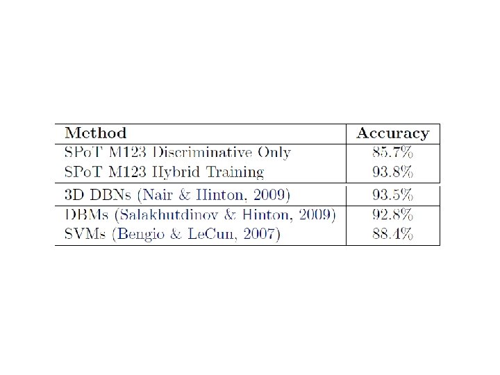
Object Recognition • The hybrid model outperformed the state of the art 3 D DBN by a small margin of 0. 3% • The fully discriminative SPo. T model overfits and only achieves a test accuracy of 85. 7% • Regularizing the model to be a generative model significantly helps the model to generalize beyond the dataset

Thank You