LBO analysis Kevin Chiang UVM Outline I APV

LBO analysis Kevin Chiang, UVM

Outline � I. APV model � II. LBO model � III. M&A premium analysis
Valuation features of an LBO � 1. A large size LBO usually has a very high debt ratio (D/(E+D)) of about 60 -70%. As time goes by, senior debt is significantly reduced, and the debt ratio at exit can be as low as 30%. � That is, debt ratio varies a lot during a typical holding horizon of 4 -6 years. � The valuation question: how can we address this dynamics in debt and time-varying WACC? � 2. Debt needs to be serviced, and this imposes a debt capacity issue; that is, the fund’s leverage has a ceiling so that it is financially feasible and sustainable. � That is, an LBO analysis requires a debt schedule that contains each year’s forecasted debt balance, interest expenses, and cash available for debt repayment.
Can we use the same WACC method? Yes, but… � The FCF discounted model introduced earlier (Topic #4: Target valuation) uses WACC as the discount rate to discount free cash flows (to the firm). � This method can be used to establish a valuation range (via sensitivity analysis) for an LBO as well with the use of some long-run debt ratio or some average debt ratio. � But, overall, the WACC method is cumbersome because debt ratio varies significantly, and thus is a less popular tool for LBO analysis. � Here, we focus on two additional methods: (1) the adjusted present value (APV) model, and (2) the LBO model. � We will also introduce a 3 rd method: M&A premium analysis.

The APV model � The main idea of the APV model is to unbundle the components of corporate value and analyzes each one separately. � EV = Present value of a levered, operating firm (VL)= present value of an all-equity (unlevered) firm (VU)+ present value of all financing/leverage effects � That is, this model views valuation creation come from two sources: (1) operations only (thus, PV of unlevered firm), and (2) financial/leverage maneuvers (thus, PV of financing/leverage effects). � Although financing effects include interest tax shield, distress costs, and others, for better or worse most analyses focus on the present value of tax shield (PVTS). If so: � VL = VU + PVTS

Recall

RJR Nabisco � For this topic, we will use the, now classics, RJR Nabisco buyout in 1988 as an illustration. � RJR Nabisco was a tobacco (about 40% of sales, but very profitable) + food businesses (not so profitable) in 1988. � “The management group” led by CEO Ross Johnson proposed a buyout at $75 per share, which is a 34% premium relative to the pre-offer share price of $55. 875. � Four days later, KKR proposed a bid of $90 a share. � The outcome of the bidding war was that KKR bought RJR Nabisco at $109 a share. � KKR would dispose some food businesses and expect asset sales proceeds of $3500 million and $2700 million in 1989 and 1990, respectively.
Step 1: Prepare pro forma � To compute FCF, we need to forecast at least the following items for each year during a standard holding horizon of 5 years: EBITDA, EBIT (thus D&A), EBIAT (thus tax rate), capex, investment in NWC, and other uses/sources of cash such as asset sales or acquisitions. � If the management’s pro forma is used, PEs usually would apply a discount to those numbers (say a 20 -25% discount to forecasted EBITDA) from the management. � Many practitioners will compile a complete set of pro forma income statements, balance sheets, and the statements of cash flows. � These forecasted numbers are then used to prepare debt repayment schedule. Note that the table of debt repayment schedule is fundamentally important for the LBO model because it is an equity-in & equity-out analysis in which the ending value of equity needs to be net out of the ending balance of debt at exit. � Debt repayment schedule is relevant to the APV model in that it helps determine interest expenses and thus the size of tax shield.
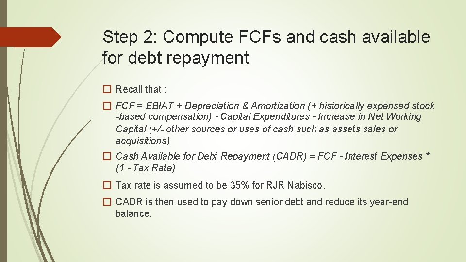
Step 2: Compute FCFs and cash available for debt repayment � Recall that : � FCF = EBIAT + Depreciation & Amortization (+ historically expensed stock -based compensation) – Capital Expenditures – Increase in Net Working Capital (+/- other sources or uses of cash such as assets sales or acquisitions) � Cash Available for Debt Repayment (CADR) = FCF – Interest Expenses * (1 – Tax Rate) � Tax rate is assumed to be 35% for RJR Nabisco. � CADR is then used to pay down senior debt and reduce its year-end balance.

Step 3: Compute unlevered beta and required unlevered/asset return �
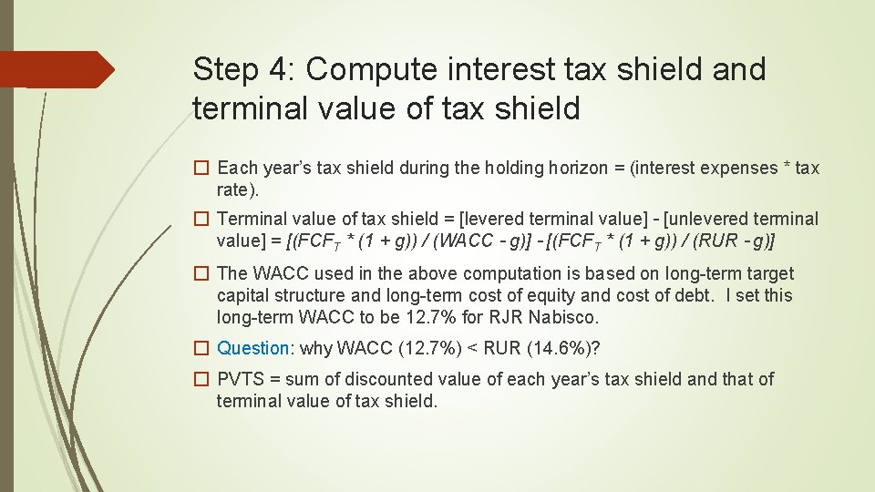
Step 4: Compute interest tax shield and terminal value of tax shield � Each year’s tax shield during the holding horizon = (interest expenses * tax rate). � Terminal value of tax shield = [levered terminal value] – [unlevered terminal value] = [(FCFT * (1 + g)) / (WACC – g)] – [(FCFT * (1 + g)) / (RUR – g)] � The WACC used in the above computation is based on long-term target capital structure and long-term cost of equity and cost of debt. I set this long-term WACC to be 12. 7% for RJR Nabisco. � Question: why WACC (12. 7%) < RUR (14. 6%)? � PVTS = sum of discounted value of each year’s tax shield and that of terminal value of tax shield.
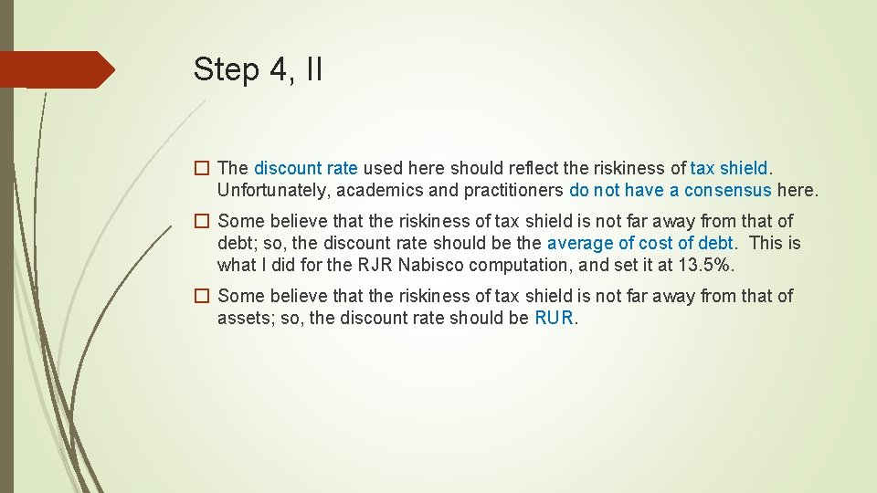
Step 4, II � The discount rate used here should reflect the riskiness of tax shield. Unfortunately, academics and practitioners do not have a consensus here. � Some believe that the riskiness of tax shield is not far away from that of debt; so, the discount rate should be the average of cost of debt. This is what I did for the RJR Nabisco computation, and set it at 13. 5%. � Some believe that the riskiness of tax shield is not far away from that of assets; so, the discount rate should be RUR.

Step 5: Compute firm value � VL = VU + PVTS � VL is the ceiling for the bid price of the target’s EV. � Adding cash on hand deducting the market value of debt (and the market value of preferred stocks) from VL yields an estimate for equity value. � Dividing equity value by the number of shares gives us an upper bound estimate of share value.

RJR Nabisco $ Million Valuation @ 12/31/88 1988 18950 E 1989 15676. 0 E 1990 12525. 0 E 1991 11461. 5 E 1992 10104. 0 E 1993 8411. 1 3500 3360 2860 11. 5% 3500 3700 3225 11. 5% 3500 4280 3805 11. 5% 3500 4610 4135 11. 5% 3500 4970 4495 11. 5% Pre-Offer Beta Tax Rate D/E Unlevered Beta 0. 97 35% 0. 6 0. 7 14% 14% 14% Risk-Free Rate 9% 2669. 3 2292. 7 1930. 4 1808. 1 1652. 0 Market Risk Premium 8% 35% 35% 35% Interest Tax Shield EBIAT 934. 2 1859 802. 5 2096. 3 675. 6 2473. 3 632. 8 2687. 8 578. 2 2921. 8 Plus: Depreciation & Amortization Less: Capex Less: investment in NWC Plus: Asset Sales Proceeds FCF 500 770 80 3500 5009 475 550 80 2700 4641. 3 475 550 80 2318. 3 2532. 8 2766. 8 Less: Net Interest Expenses after Tax 1735. 0 1490. 3 1254. 7 1175. 3 1073. 8 Cash Available for Debt Repayment Unlevered Terminal Value PV Total Unlevered Value Levered Terminal Value of Tax Shield @ Exit PV Total Tax Shield Value EV (Total Levered Value) Cash on Hand MV of Pre-Offer Debt Equity Value # Shares Share Value 3274. 0 3151. 0 1063. 5 1357. 5 4370. 9 3534. 0 1540. 3 1468. 4 1693. 0 24566. 8 13828. 4 381. 3 29378. 9 4812. 1 2861. 7 New. Co Bank Debt Balance New. Co Subordinated Debt Balance EBITDA EBIT Interest Rate: Bank Debt Interest Rate: Subordinated Debt Interest Expenses Tax Rate 24742. 0 823. 1 5151. 2 29893. 2 1000. 0 4300 26593. 2 229 116. 1 622. 9 462. 1 Required Asset Return 14. 6% Average Cost of Debt L-T Growth Rate 13. 5% 3% L-T WACC 12. 7%
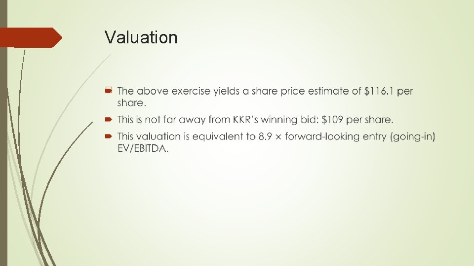
Valuation �

Buy-side and sell-side advisors � KKR hired Morgan Stanley, Wasserstein, Perella & Co. , Drexel Burnham Lambert & Co. , and Merrill Lynch to assist its financing. � Lazard and Dillon, Reed & Co. were hired by RJR Nabisco as its advisors. The sell-side advisors’ valuation of RJR Nabisco under the KKR plan was $108 per share.
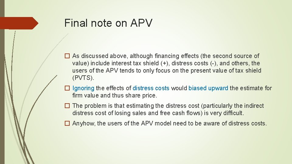
Final note on APV � As discussed above, although financing effects (the second source of value) include interest tax shield (+), distress costs (-), and others, the users of the APV tends to only focus on the present value of tax shield (PVTS). � Ignoring the effects of distress costs would biased upward the estimate for firm value and thus share price. � The problem is that estimating the distress cost (particularly the indirect distress cost of losing sales and free cash flows) is very difficult. � Anyhow, the users of the APV model need to be aware of distress costs.

The LBO model � The APV model (a member of DCF models) is used to generate value estimates for EV, equity value, and share value. � The APV method has not been widely used by practitioners yet. Gompers et al. (2016, JFE) find that less than 20% of PE practitioners use a DCF method. � The LBO model is used to estimate the gross IRR of the deal (i. e. , at the investment level). � According to Gompers et al. (2016), the LBO model is used by 90% of practitioners. � This estimated (gross) IRR will be compared to the “deal” (not fund) hurdle rate (usually 25 -30%), and the deal will be accepted (rejected) if the computed (gross) IRR is greater (less) than the hurdle rate.
Step 1: Repeat the first two steps of the APV method � That is, first perform pro forma. � Next, estimate FCFs and cash available for debt repayment so that debt schedule throughout the holding horizon is derived.
Step 2: Terminal value determination; Forecast EV/EBITDA multiples for entry and exit � Use pro forma EBITDA and the assumed multiples to estimate the entry EV and the exit EV (terminal value). Alternatively, the growing perpetuity method can be used. � Gompers et al. (2016, JFE) find that about 2/3 of practitioners use a multiple method to estimate terminal value, and about 1/3 of practitioners use growing perpetuity DCF method (like the one that we used in the APV model discussion) to estimate terminal value. � With information on pre-offer debt balance, pre-offer cash on hand, exit debt balance, and maybe exit cash on hand, we can compute equity-in at entry and equity-out at exit. � (Gross) IRR then can be computed based on equity-in and equity-out.
Step 3: Sensitivity analysis � The resulting IRR estimate is very sensitive to the choice of entry multiple and that of exit multiple. � While sponsors can observe the current market conditions and usually have a rather good sense about what entry multiple is likely to incur, they may suffer the winner’s curse when there is a intense competition (e. g. , bidding war) among potential acquirers. � All other things being equal, the more one pays for the target, the less the IRR. � The realization of exit multiple is many years down the road, and has high uncertainty. � Thus, a careful sensitivity analysis on exit multiple is particularly important.

RJR Nabisco Valuation @ 12/31/88 $ Million 1988 E 1989 E 1990 E 1991 E 1992 E 1993 18950 15676. 0 12525. 0 11461. 5 10104. 0 8411. 1 3500 3500 EBITDA 3360 3700 4280 4610 4970 EBIT 2860 3225 3805 4135 4495 11. 5% 14% 14% 14% 2669. 3 2292. 7 1930. 4 1808. 1 1652. 0 35% 35% 35% New. Co Bank Debt Balance New. Co Subordinated Debt Balance Interest Rate: Bank Debt Interest Rate: Subordinated Debt Interest Expenses Tax Rate Interest Tax Shield 934. 2 802. 5 675. 6 632. 8 578. 2 EBIAT 1859 2096. 3 2473. 3 2687. 8 2921. 8 Plus: Depreciation & Amortization 500 475 475 Less: Capex 770 550 550 80 80 80 Less: investment in NWC Plus: Asset Sales Proceeds 3500 2700 FCF 5009 4641. 3 2318. 3 2532. 8 2766. 8 1735. 0 1490. 3 1254. 7 1175. 3 1073. 8 3274. 0 3151. 0 1063. 5 1357. 5 1693. 0 Less: Net Interest Expenses after Tax Cash Available for Debt Repayment Entry Multiple Exit Multiple EV Cash 8. 9 Exit Multiple IRR 29904 8. 9 8. 4 30. 90% 46992 1000 8. 9 32. 90% 0 MV of Debt 22450 9. 4 34. 90% 11911. 1 Equity-In (-) and Equity-Out (+) -8454 # Shares 229 Share Price 36. 9 IRR 32. 9% 0 0 35080. 9 E 1994 5280
Notes � The above analysis ignore transactions costs and fees to advisors, underwriters, accountants, attorney, etc. If the fees were taken into consideration, they will increase equity-in and reduces gross IRR. � This estimated gross IRR, 32. 9%, is the IRR at the deal level. Note that this is not the net IRR to LPs at the fund level. � As noted in the previous topic (Topic #6: Private Equity), management fees and carry usually take away about 5% of the gross IRR. � Thus, if the deal-level transactions costs and fees and GP’s compensation are accounted for, the net IRR to LPs could be reduced to around 20 -25%. � Sensitivities: also note that the gross IRR varies a lot (30. 9 -34. 9%) when exit multiple reduces/increases by 0. 5 from 8. 9 to 8. 4/9. 4.

Q&As � Q: After running an LBO model/analysis, you notice that the return (gross IRR) of the proposed deal is too low. What drivers to (variables of) the model will increase the return? � A: (1) Reducing the purchase price, (2) increasing the exit EV (via a higher exit multiple or a higher growth rate), (3) increasing the amount of debt (leverage), and (4) raising the FCF (along with EBITDA, etc. ) estimates during the projection period. � Q: What is IRR and how does it differ from WACC? � A: In general, IRR is the “expected” rate of return each year for capital providers. WACC is the “required” rate of return each year demanded by capital providers for bearing investment risks. For LBO analysis, the gross IRR is the “expected” (not required) rate of return each year during the investment horizon for equity investors (LPs) before management fee and carry.
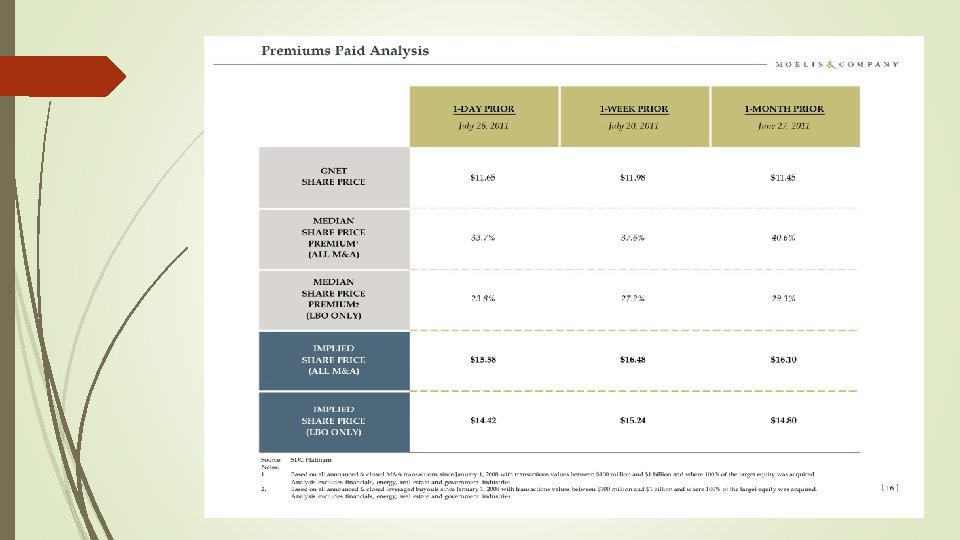
M&A premium analysis � This is an extension of the deal comp. � It looks into similar (same industry, past 2 -3 years, similar sizes, etc. ) precedent transactions and see the premiums that previous winning bidders had paid. It then applies the historical median (average) premium to the target’s recent stock prices to arrive at a valuation estimate. � This analysis can be perform for the premiums based on the target’s share price 1 day, 1 week, and 1 month (or different time intervals) before the transaction was announced. � A range of share prices over a range of dates is used because the deal may be leaked or anticipated. � The following example of the M&A premium analysis is from the next topic: M&As.
General Qs � Q: Walk me through an APV valuation. � Q: Walk me through an LBO analysis. � Q: Walk me through a premium analysis for an acquisition.
- Slides: 27