Latent Growth Curve Modeling using Mplus Richard N

Latent Growth Curve Modeling using Mplus Richard N. Jones, Sc. D. Hebrew Rehabilitation Center for Aged Research and Training Institute Boston, MA University of Washington Psychometrics Workshop September 20 -25, 2004 Please send questions and corrections to jones@mail. hrca. harvard. edu 1

Overview of this talk • Other Resources • Statistical model • Implementation in Mplus • Example • Discussion – Limitations – Advantages • Mplus (www. statmodel. com) 2

Other Resources (Don’t take my word for it) Curran, P. (2000). A latent curve framework for the study of developmental trajectories in adolescent substance use. In J. Rose, L. Chassin, C. Presson & J. Sherman (Eds. ), Multivariate Applications in Substance Use Research. Hillsdale, NJ: Lawrence Erlbaum Associates. Curran, P. J. , & Muthén, B. (1996). Testing developmental theories in intervention research: latent growth analysis and power estimation. Los Angeles: Graduate School of Education and Information Studies, University of California, Los Angeles. Muthén, B. , Brown, C. H. , Masyn, K. , Jo, B. , Khoo, S. -T. , Yang, C. -C. , et al. (2002). General growth mixture modeling for randomized preventive interventions. Biostatistics, 3(4), 459 -475. Muthén, B. , & Curran, P. (1997). General growth modeling in experimental designs: A latent variable framework for analysis and power estimation (CSE Technical Report No. 443): National Center for Research and Evalation, Standards and Student Testing (CRESST)/Graduate School of Education & Information Studies, University of California, Los Angeles. Muthén, B. , & Curran, P. (1997). General longitudinal modeling of individual differences in experimental designs: a latent variable framework for analysis and power estimation. Psychological Methods, 2(4), 371 -402. Muthén, B. O. (1998 -2004). Mplus Technical Appendices. Los Angeles, CA: Muthén & Muthén, L. K. , & Muthén, B. O. (1998 -2003). Mplus users guide (February 2001, Version 2 ed. ). Los Angeles, CA: Muthén & Muthén. Mplus Short Courses (November 2004, Alexandria VA) see www. statmodel. com Also see Jones, R. N. , Allaire, J. , Mc. Coy, K. , Kleinman, K. , Rebok, G. , Malloy, P. , et al. (2004). A growth curve model of learning acquisition among cognitively normal older adults. Experimental Aging Research, in press. 3

Implementing LGM Models in Mplus • Mplus has capabilities of popular SEM software packages (LISREL, EQS, AMOS) • Mplus has unique features, e. g. – Random effects for individually-varying times of observations – Easy modeling of mean structures (thresholds, means) – Also • Latent class and mixture modeling • Regression based treatment of exogenous variables (covariates) • These special features make modeling change easy 4

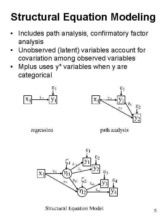
Structural Equation Modeling • Includes path analysis, confirmatory factor analysis • Unobserved (latent) variables account for covariation among observed variables • Mplus uses y* variables when y are categorical 5

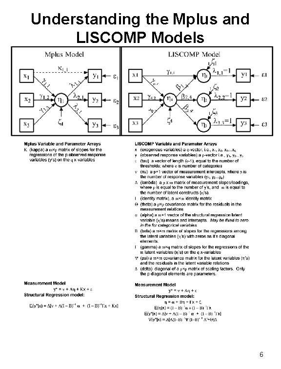
Understanding the Mplus and LISCOMP Models 6

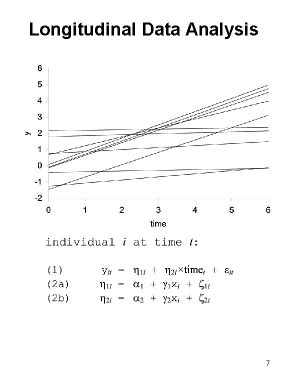
Longitudinal Data Analysis 7

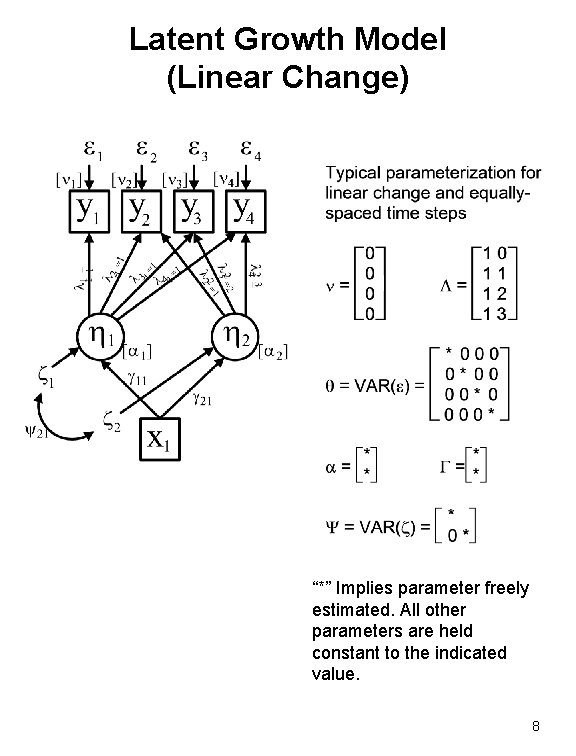
Latent Growth Model (Linear Change) “*” Implies parameter freely estimated. All other parameters are held constant to the indicated value. 8

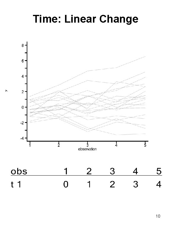
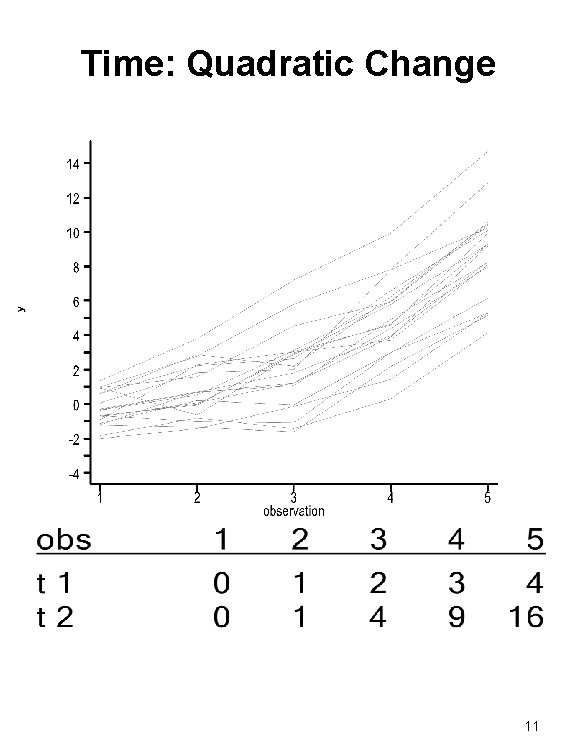
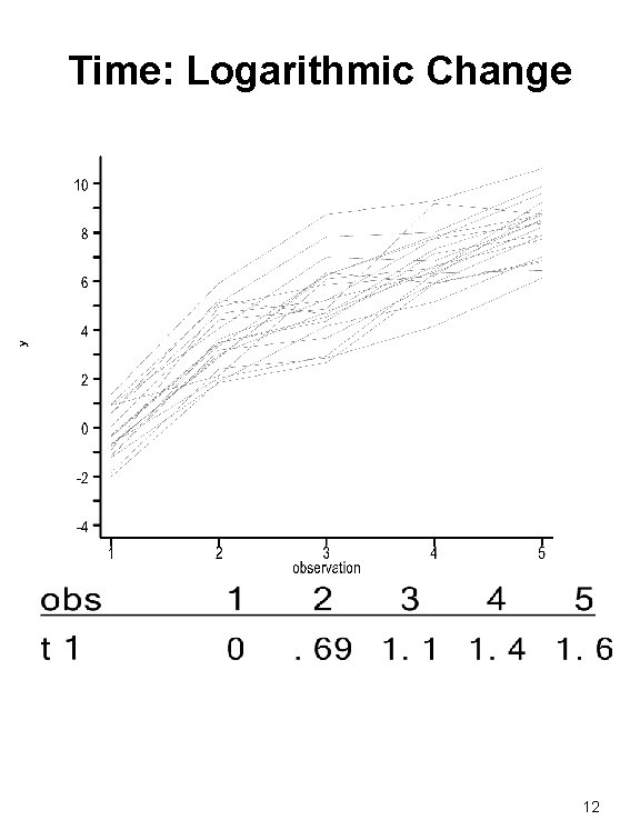
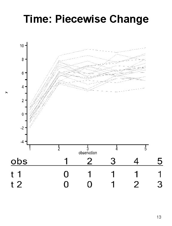
Be Eclectic in Treatment of Time Dimension • Changes over time vs. changes with age • Changes over time/age vs. disease progression • Functional form of changes – Linear – Quadratic – Logarithmic – Piecewise 9

Time: Linear Change 10

Time: Quadratic Change 11

Time: Logarithmic Change 12

Time: Piecewise Change 13

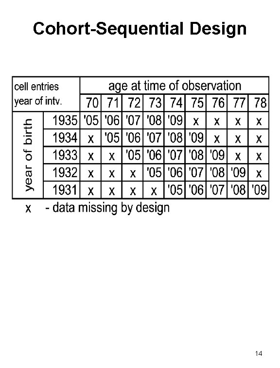
Cohort-Sequential Design 14

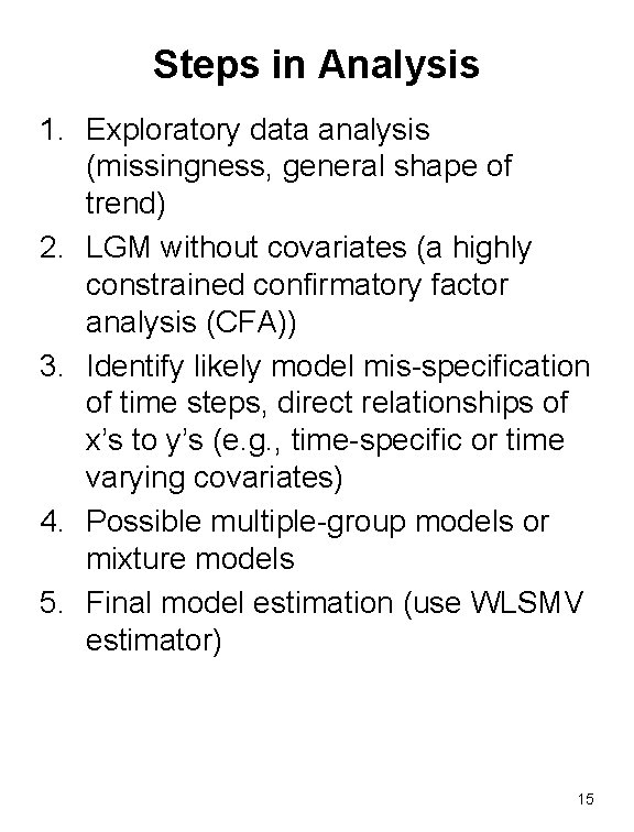
Steps in Analysis 1. Exploratory data analysis (missingness, general shape of trend) 2. LGM without covariates (a highly constrained confirmatory factor analysis (CFA)) 3. Identify likely model mis-specification of time steps, direct relationships of x’s to y’s (e. g. , time-specific or time varying covariates) 4. Possible multiple-group models or mixture models 5. Final model estimation (use WLSMV estimator) 15

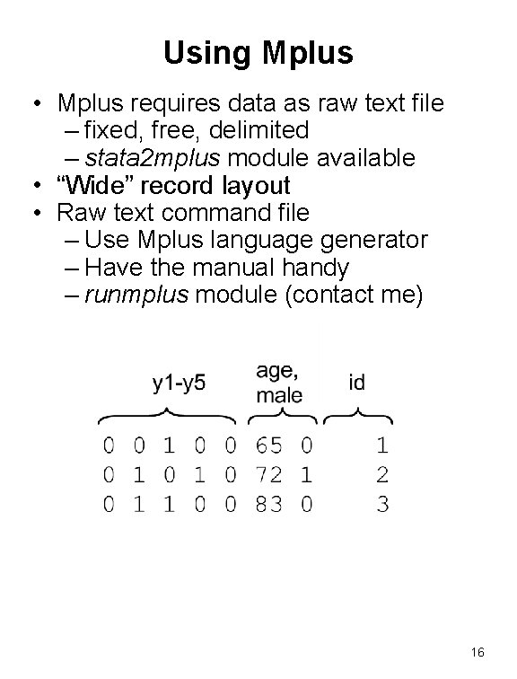
Using Mplus • Mplus requires data as raw text file – fixed, free, delimited – stata 2 mplus module available • “Wide” record layout • Raw text command file – Use Mplus language generator – Have the manual handy – runmplus module (contact me) 16

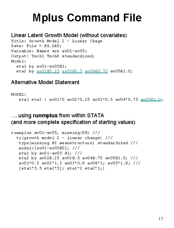
Mplus Command File Linear Latent Growth Model (without covariates) Title: Growth Model 2 – Linear Chage Data: File = EX. DAT; Variable: Names are av 01 -av 05; Output: Tech 1 Tech 8 standardized; Model: eta 1 by av 01 -av 05@1; eta 2 by av 02@0. 25 av 03@0. 5 av 04@0. 75 av 05@1. 0; Alternative Model Statement MODEL: eta 1 eta 2 | av 01*0 av 02*0. 25 av 03*0. 5 av 04*0. 75 av 05@1. 0; . . . using runmplus from within STATA (and more complete specification of starting values) runmplus av 01 -av 05, missing(99) /// ti(growth model 2 - linear change) /// type(missing H 1 meanstructure) standardized /// model([av 01 -av 05@0]; /// eta 1 by av 01 -av 05 @1; /// eta 2 by av 02@. 25 av 03@. 5 av 04@. 75 av 05@1. 0; /// av 01*0. 5 av 02*1. 3 av 03*0. 9 av 04*1; av 05*1. 9; /// [eta 1*5. 5 eta 2*5]; eta 1*2 eta 2*1; ) 17

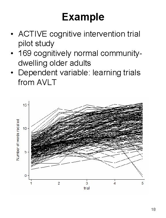
Example • ACTIVE cognitive intervention trial pilot study • 169 cognitively normal communitydwelling older adults • Dependent variable: learning trials from AVLT 18

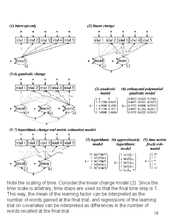
Note the scaling of time. Consider the linear change model (2). Since the time scale is arbitrary, time steps are used so that the final time step is 1. This way, the mean of the learning factor can be interpreted as the number of words gained at the final trial, and regressions of the learning trial on covariates can be interpreted as differences in the number of words recalled at the final trial. 19

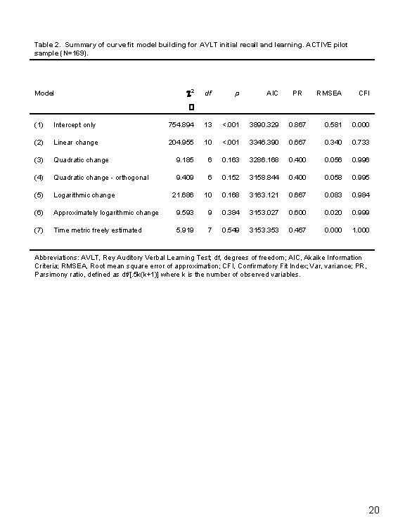
Table 2. Summary of curve fit model building for AVLT initial recall and learning. ACTIVE pilot sample (N=169). Model c 2 df p AIC PR RMSEA CFI � (1) Intercept only 754. 894 13 <. 001 3890. 329 0. 867 0. 581 0. 000 (2) Linear change 204. 955 10 <. 001 3346. 390 0. 667 0. 340 0. 733 (3) Quadratic change 9. 185 6 0. 163 3286. 168 0. 400 0. 056 0. 996 (4) Quadratic change - orthogonal 9. 409 6 0. 152 3158. 844 0. 400 0. 058 0. 995 (5) Logarithmic change 21. 686 10 0. 168 3163. 121 0. 667 0. 083 0. 984 (6) Approximately logarithmic change 9. 593 9 0. 384 3153. 027 0. 600 0. 020 0. 999 (7) Time metric freely estimated 5. 919 7 0. 549 3153. 353 0. 467 0. 000 1. 000 Abbreviations: AVLT, Rey Auditory Verbal Learning Test; df, degrees of freedom; AIC, Akaike Information Criteria; RMSEA, Root mean square error of approximation; CFI, Confirmatory Fit Index; Var, variance; PR, Parsimony ratio, defined as df/[. 5 k(k+1)] where k is the number of observed variables. 20

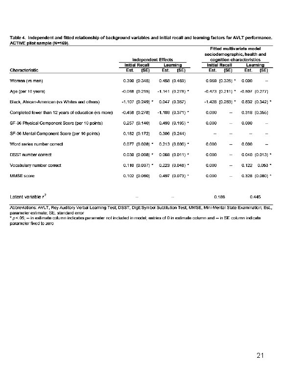
21

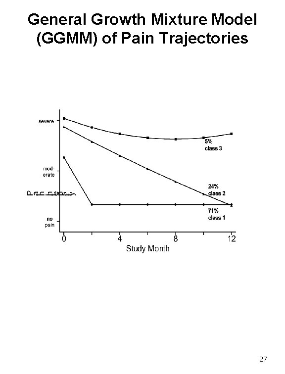
Example 2: General Growth Mixture Modeling (GGMM) The Course of Pain Following Fall or Fracture Among Residents of Long-Term Care RN Jones, A Won Supported by Harvard Older Americans Independence Center (2 P 60 AG 008812), 22

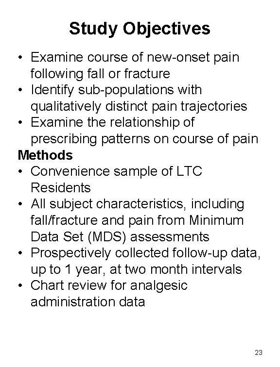
Study Objectives • Examine course of new-onset pain following fall or fracture • Identify sub-populations with qualitatively distinct pain trajectories • Examine the relationship of prescribing patterns on course of pain Methods • Convenience sample of LTC Residents • All subject characteristics, including fall/fracture and pain from Minimum Data Set (MDS) assessments • Prospectively collected follow-up data, up to 1 year, at two month intervals • Chart review for analgesic administration data 23

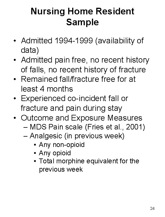
Nursing Home Resident Sample • Admitted 1994 -1999 (availability of data) • Admitted pain free, no recent history of falls, no recent history of fracture • Remained fall/fracture free for at least 4 months • Experienced co-incident fall or fracture and pain during stay • Outcome and Exposure Measures – MDS Pain scale (Fries et al. , 2001) – Analgesic (in previous week) • Any non-opioid • Any opioid • Total morphine equivalent for the previous week 24

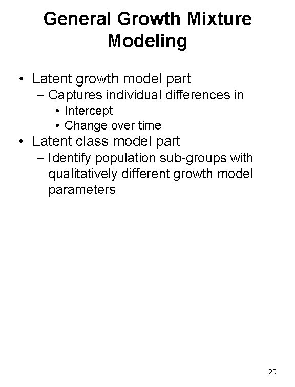
General Growth Mixture Modeling • Latent growth model part – Captures individual differences in • Intercept • Change over time • Latent class model part – Identify population sub-groups with qualitatively different growth model parameters 25

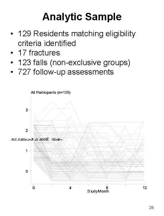
Analytic Sample • 129 Residents matching eligibility criteria identified • 17 fractures • 123 falls (non-exclusive groups) • 727 follow-up assessments 26

General Growth Mixture Model (GGMM) of Pain Trajectories 27

Discussion • Advantages – Regressions among random coefficients (growth factors) – Multiple Processes – Multiple Indicators • IRT model for outcome dimension • Growth model for latent trait • Model DIF item difficulty shifts – Multiple Populations – Embed within larger SEM – – • LGM with discrete time survival model to simultaneously model change and survival ‘Easy’ inclusion of time-varying covariates Growth Mixture Modeling ‘Simple’ power calculation Maximum likelihood estimation with missing data – Adjustment for complex sampling design – Modeling with a preponderance of 0’s and/or censored data • Disadvantages – Individually-varying times of observation (Mplus versus other SEM software) 28

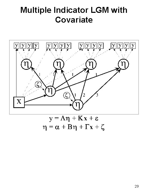
Multiple Indicator LGM with Covariate 29

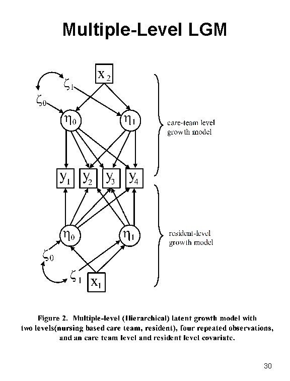
Multiple-Level LGM 30

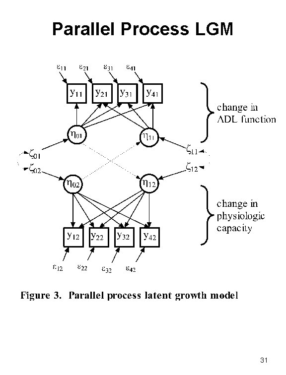
Parallel Process LGM 31

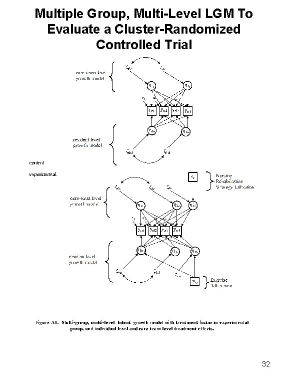
Multiple Group, Multi-Level LGM To Evaluate a Cluster-Randomized Controlled Trial 32