Lateness Models Contents 1 Lawlers algorithm which gives

Lateness Models Contents 1. Lawler’s algorithm which gives an optimal schedule with the minimum cost hmax when the jobs are subject to precedence relationship 1 | prec | hmax 2. A branch-and-bound algorithm for the scheduling problems with the objective to minimise lateness 1 | rj | Lmax Literature: • Scheduling, Theory, Algorithms, and Systems, Michael Pinedo, Prentice Hall, 1995, Chapter 3. 2 1 or new: Second Addition, 2002, Chapter 3.

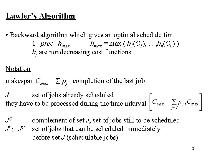
Lawler’s Algorithm • Backward algorithm which gives an optimal schedule for 1 | prec | hmax = max ( h 1(C 1), . . . , hn(Cn) ) hj are nondecreasing cost functions Notation makespan Cmax = pj completion of the last job J set of jobs already scheduled they have to be processed during the time interval JC J' JC complement of set J, set of jobs still to be scheduled set of jobs that can be scheduled immediately before set J (schedulable jobs) 2

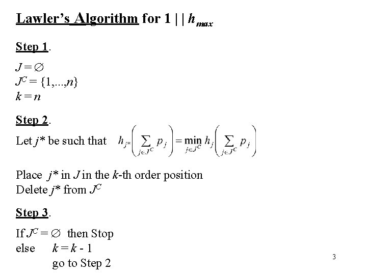
Lawler’s Algorithm for 1 | | hmax Step 1. J= JC = {1, . . . , n} k=n Step 2. Let j* be such that Place j* in J in the k-th order position Delete j* from JC Step 3. If JC = then Stop else k = k - 1 go to Step 2 3

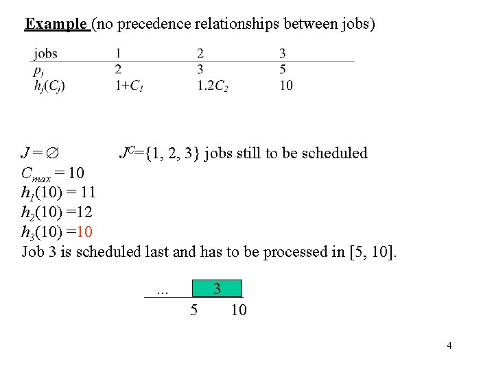
Example (no precedence relationships between jobs) J= JC={1, 2, 3} jobs still to be scheduled Cmax = 10 h 1(10) = 11 h 2(10) =12 h 3(10) =10 Job 3 is scheduled last and has to be processed in [5, 10]. 3 . . . 5 10 4

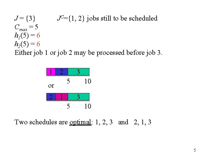
J = {3} JC={1, 2} jobs still to be scheduled Cmax = 5 h 1(5) = 6 h 2(5) = 6 Either job 1 or job 2 may be processed before job 3. 1 2 5 or 2 3 1 10 3 5 10 Two schedules are optimal: 1, 2, 3 and 2, 1, 3 5

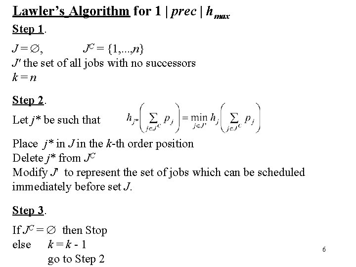
Lawler’s Algorithm for 1 | prec | hmax Step 1. J = , JC = {1, . . . , n} J' the set of all jobs with no successors k=n Step 2. Let j* be such that Place j* in J in the k-th order position Delete j* from JC Modify J' to represent the set of jobs which can be scheduled immediately before set J. Step 3. If JC = then Stop else k = k - 1 go to Step 2 6

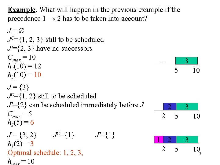
Example. What will happen in the previous example if the precedence 1 2 has to be taken into account? J= JC={1, 2, 3} still to be scheduled J'={2, 3} have no successors Cmax = 10 h 2(10) = 12 h 3(10) = 10 5 J = {3} JC={1, 2} still to be scheduled J'={2} can be scheduled immediately before J Cmax = 5 h 2(5) = 6 J = {3, 2} JC={1} h 1(2) = 3 Optimal schedule: 1, 2, 3, h = 10 J'={1} 3 . . . 2 2 1 3 5 2 2 10 10 3 5 10 7

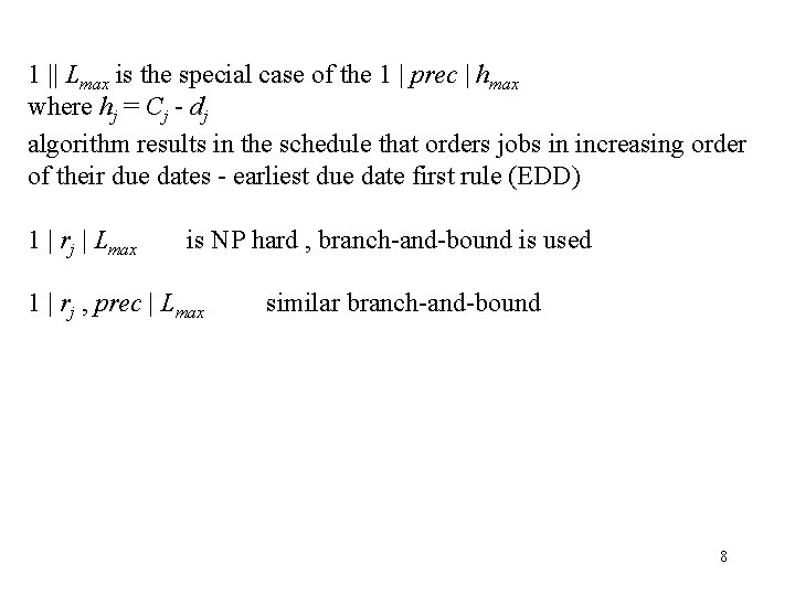
1 || Lmax is the special case of the 1 | prec | hmax where hj = Cj - dj algorithm results in the schedule that orders jobs in increasing order of their due dates - earliest due date first rule (EDD) 1 | rj | Lmax is NP hard , branch-and-bound is used 1 | rj , prec | Lmax similar branch-and-bound 8

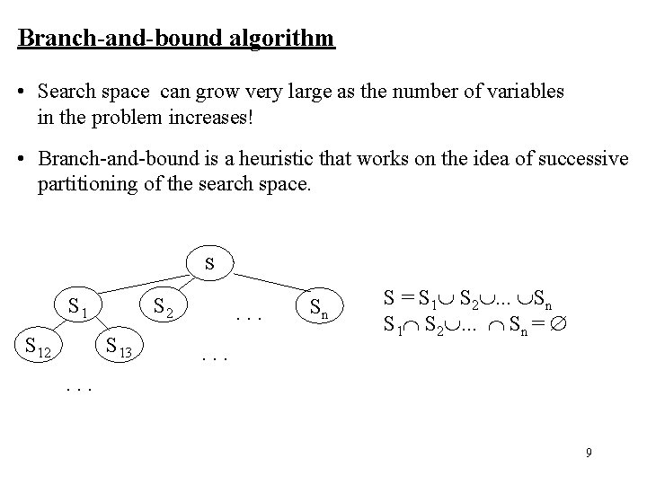
Branch-and-bound algorithm • Search space can grow very large as the number of variables in the problem increases! • Branch-and-bound is a heuristic that works on the idea of successive partitioning of the search space. S S 12 S 13 . . . Sn S = S 1 S 2. . . Sn = . . . 9

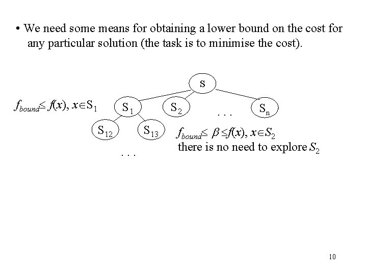
• We need some means for obtaining a lower bound on the cost for any particular solution (the task is to minimise the cost). S fbound f(x), x S 1 S 12 S 13 . . . Sn fbound f(x), x S 2 there is no need to explore S 2 10

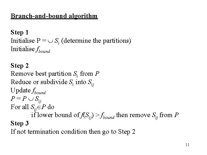
Branch-and-bound algorithm Step 1 Initialise P = Si (determine the partitions) Initialise fbound Step 2 Remove best partition Si from P Reduce or subdivide Si into Sij Update fbound P = P Sij For all Sij P do if lower bound of f(Sij) > fbound then remove Sij from P Step 3 If not termination condition then go to Step 2 11

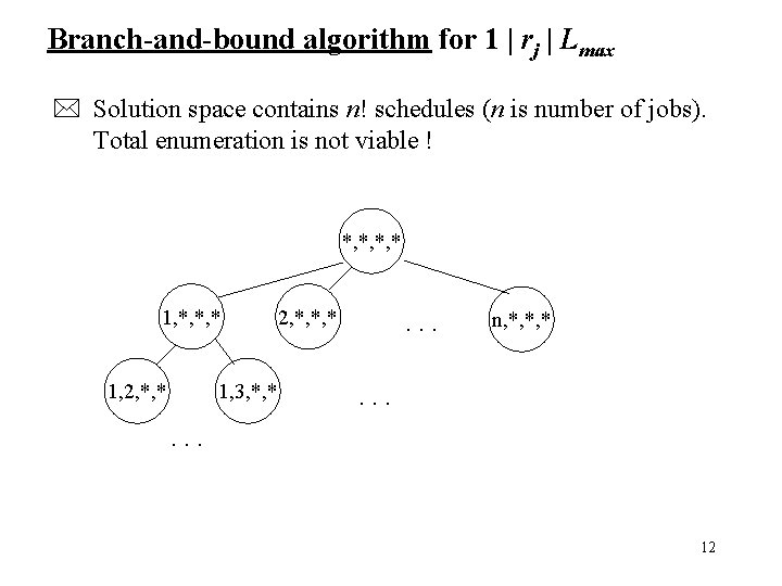
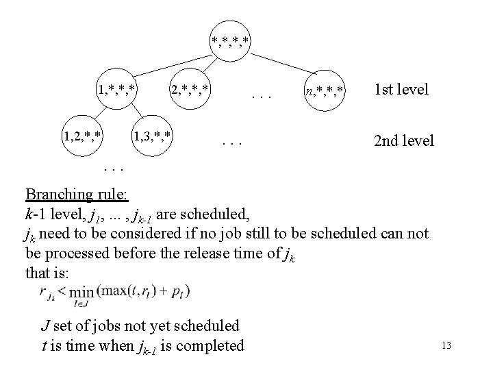
Branch-and-bound algorithm for 1 | rj | Lmax * Solution space contains n! schedules (n is number of jobs). Total enumeration is not viable ! *, *, *, * 1, 2, *, * 1, 3, *, * 2, *, *, * . . . n, *, *, * . . . 12

*, *, *, * 1, 2, *, * 1, 3, *, * 2, *, *, * . . . n, *, *, * 1 st level 2 nd level . . . Branching rule: k-1 level, j 1, . . . , jk-1 are scheduled, jk need to be considered if no job still to be scheduled can not be processed before the release time of jk that is: J set of jobs not yet scheduled t is time when jk-1 is completed 13

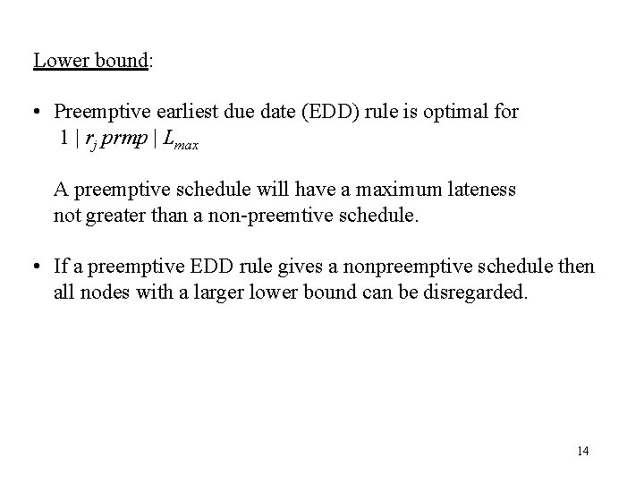
Lower bound: • Preemptive earliest due date (EDD) rule is optimal for 1 | rj prmp | Lmax A preemptive schedule will have a maximum lateness not greater than a non-preemtive schedule. • If a preemptive EDD rule gives a nonpreemptive schedule then all nodes with a larger lower bound can be disregarded. 14

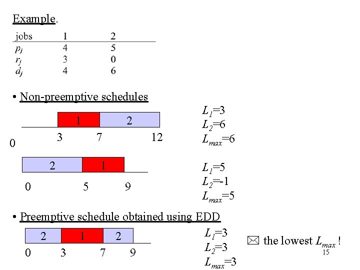
Example. • Non-preemptive schedules 1 2 3 0 2 0 12 7 1 5 9 L 1=3 L 2=6 Lmax=6 L 1=5 L 2=-1 Lmax=5 • Preemptive schedule obtained using EDD L 1=3 2 1 2 * the lowest Lmax ! L =3 2 15 0 3 7 9 Lmax=3

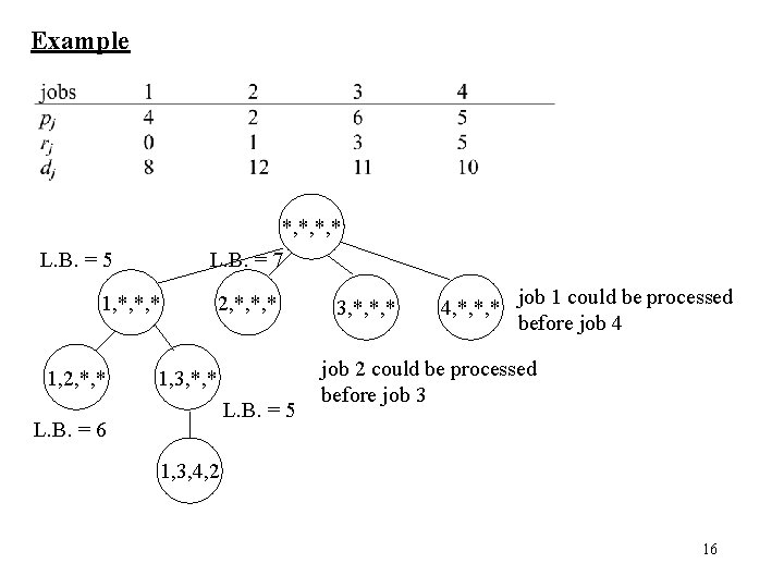
Example *, *, *, * L. B. = 7 L. B. = 5 1, *, *, * 1, 2, *, *, * 1, 3, *, * L. B. = 5 L. B. = 6 3, *, *, * 4, *, *, * job 1 could be processed before job 4 job 2 could be processed before job 3 1, 3, 4, 2 16

*, *, *, * 1 [0, 4] 3 [4, 5] 4 [5, 10] 3 [10, 15] 2 [15, 17] 1, 2, *, * 1 [0, 4] 2 [4, 6] 4 [6, 11] 3 [11, 17] L 1=-4 L 4=0 L 3=4 L 2=5 L 1=-4 L 2=-6 L 4=1 L 3=6 2, *, *, * 2 [1, 3] 1 [3, 7] 4 [7, 12] 3 [12, 18] L 2=-9 L 1=-1 L 4=2 L 3=7 1, 3, *, * 1 [0, 4] 3 [4, 10] 4 [10, 15] 2 [15, 17] L 1=-4 L 3=-1 L 4=5 L 3=5 4, *, *, * either job 1 or 2 can be processed before 4 ! 3, *, *, * job 2 can be processed before 3 ! Schedule: 1, 3, 4, 2, 17

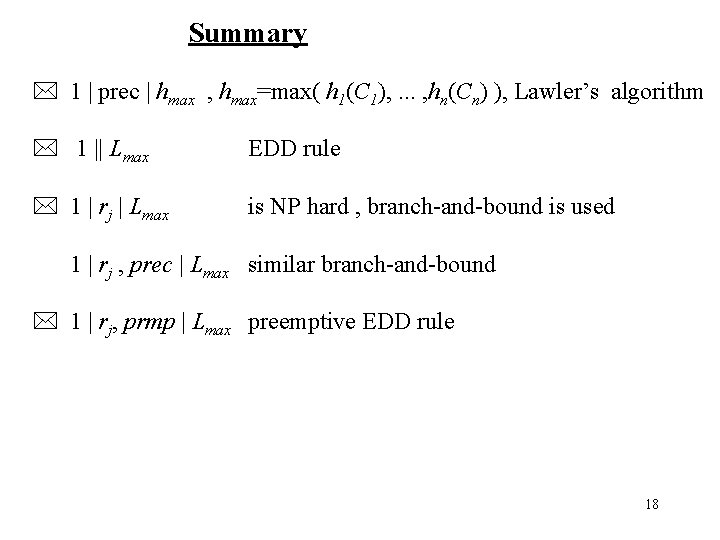
Summary * 1 | prec | hmax , hmax=max( h 1(C 1), . . . , hn(Cn) ), Lawler’s algorithm * 1 || Lmax EDD rule * 1 | rj | Lmax is NP hard , branch-and-bound is used 1 | rj , prec | Lmax similar branch-and-bound * 1 | rj, prmp | Lmax preemptive EDD rule 18