Last Time Parametric Curves Splines Hermite curves Bezier

Last Time • Parametric Curves (Splines) – Hermite curves – Bezier curves – Brief mentions of rational curves, transforming between representation, subdivision for Bezier • Homework 7 due Thursday 12/7/2004 © University of Wisconsin, CS 559 Fall 2004

Today • Parametric surface patches • Bsplines 12/7/2004 © University of Wisconsin, CS 559 Fall 2004

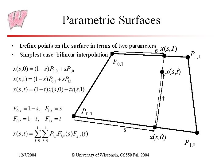
Parametric Surfaces • Define points on the surface in terms of two parameters x(s, 1) s • Simplest case: bilinear interpolation P 0, 1 P 1, 1 x(s, t) t P 0, 0 s 12/7/2004 © University of Wisconsin, CS 559 Fall 2004 x(s, 0) P 1, 0

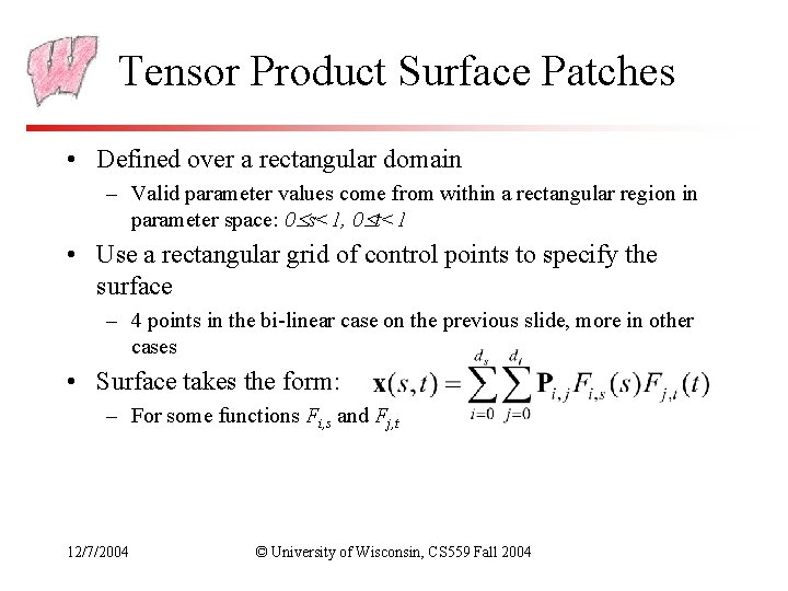
Tensor Product Surface Patches • Defined over a rectangular domain – Valid parameter values come from within a rectangular region in parameter space: 0 s<1, 0 t<1 • Use a rectangular grid of control points to specify the surface – 4 points in the bi-linear case on the previous slide, more in other cases • Surface takes the form: – For some functions Fi, s and Fj, t 12/7/2004 © University of Wisconsin, CS 559 Fall 2004

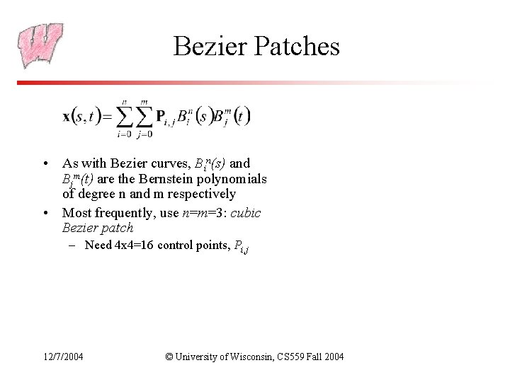
Bezier Patches • As with Bezier curves, Bin(s) and Bjm(t) are the Bernstein polynomials of degree n and m respectively • Most frequently, use n=m=3: cubic Bezier patch – Need 4 x 4=16 control points, Pi, j 12/7/2004 © University of Wisconsin, CS 559 Fall 2004

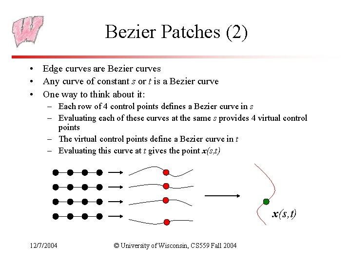
Bezier Patches (2) • Edge curves are Bezier curves • Any curve of constant s or t is a Bezier curve • One way to think about it: – Each row of 4 control points defines a Bezier curve in s – Evaluating each of these curves at the same s provides 4 virtual control points – The virtual control points define a Bezier curve in t – Evaluating this curve at t gives the point x(s, t) 12/7/2004 © University of Wisconsin, CS 559 Fall 2004

Properties of Bezier Patches • Which vertices, if any, does the patch interpolate? Why? • What can you say about the tangent plane at each corner? Why? • Does the patch lie within the convex hull of its control vertices? 12/7/2004 © University of Wisconsin, CS 559 Fall 2004

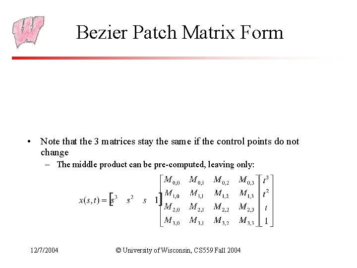
Bezier Patch Matrix Form • Note that the 3 matrices stay the same if the control points do not change – The middle product can be pre-computed, leaving only: 12/7/2004 © University of Wisconsin, CS 559 Fall 2004

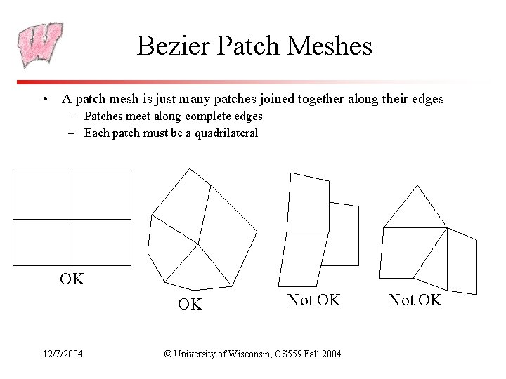
Bezier Patch Meshes • A patch mesh is just many patches joined together along their edges – Patches meet along complete edges – Each patch must be a quadrilateral OK OK 12/7/2004 Not OK © University of Wisconsin, CS 559 Fall 2004 Not OK

Bezier Mesh Continuity • Just like curves, the control points must satisfy constraints to ensure parametric continuity – How do we ensure C 0 continuity along an edge? – How do we ensure C 1 continuity along an edge? – How do we ensure C 2 continuity along an edge? • For geometric continuity, constraints are less rigid • What can you say about the vertices around a corner if there must be C 1 continuity at the corner point? 12/7/2004 © University of Wisconsin, CS 559 Fall 2004

Rendering Bezier Patches • Option 1: Evaluate at fixed set of parameter values and join up with triangles – – Can’t use quadrilaterals because points may not be co-planar Ideal situation for triangle strips Advantage: Simple, and Open. GL has commands to do it for you Disadvantage: No easy way to control quality of appearance • Option 2: Subdivision – Allows control of error in the triangle approximation – Extend 1 D curve subdivision to do surfaces – Similar to other subdivision schemes we’ve seen 12/7/2004 © University of Wisconsin, CS 559 Fall 2004

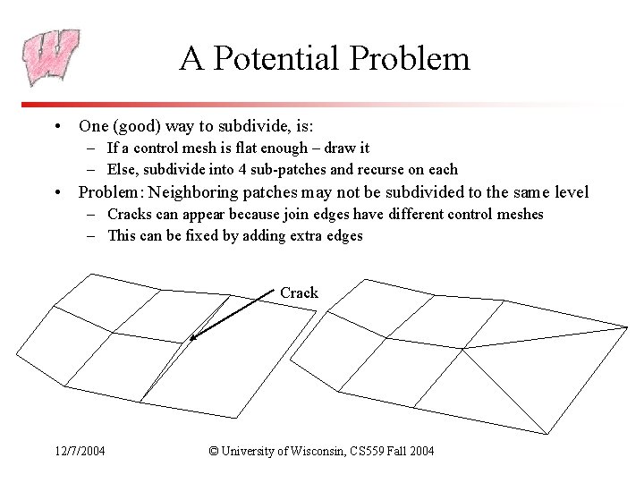
A Potential Problem • One (good) way to subdivide, is: – If a control mesh is flat enough – draw it – Else, subdivide into 4 sub-patches and recurse on each • Problem: Neighboring patches may not be subdivided to the same level – Cracks can appear because join edges have different control meshes – This can be fixed by adding extra edges Crack 12/7/2004 © University of Wisconsin, CS 559 Fall 2004

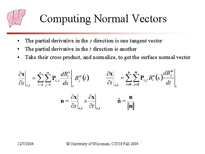
Computing Normal Vectors • The partial derivative in the s direction is one tangent vector • The partial derivative in the t direction is another • Take their cross product, and normalize, to get the surface normal vector 12/7/2004 © University of Wisconsin, CS 559 Fall 2004

Bezier Curve/Surface Problems • To make a long continuous curve with Bezier segments requires using many segments – Same for large surface • Maintaining continuity requires constraints on the control point positions – The user cannot arbitrarily move control vertices and automatically maintain continuity – The constraints must be explicitly maintained – It is not intuitive to have control points that are not free 12/7/2004 © University of Wisconsin, CS 559 Fall 2004

B-splines • B-splines automatically take care of continuity, with exactly one control vertex per curve segment • Many types of B-splines: degree may be different (linear, quadratic, cubic, …) and they may be uniform or nonuniform – We will only look closely at uniform B-splines • With uniform B-splines, continuity is always one degree lower than the degree of each curve piece – Linear B-splines have C 0 continuity, cubic have C 2, etc 12/7/2004 © University of Wisconsin, CS 559 Fall 2004

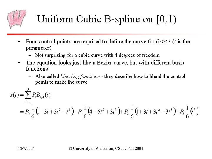
Uniform Cubic B-spline on [0, 1) • Four control points are required to define the curve for 0 t<1 (t is the parameter) – Not surprising for a cubic curve with 4 degrees of freedom • The equation looks just like a Bezier curve, but with different basis functions – Also called blending functions - they describe how to blend the control points to make the curve 12/7/2004 © University of Wisconsin, CS 559 Fall 2004

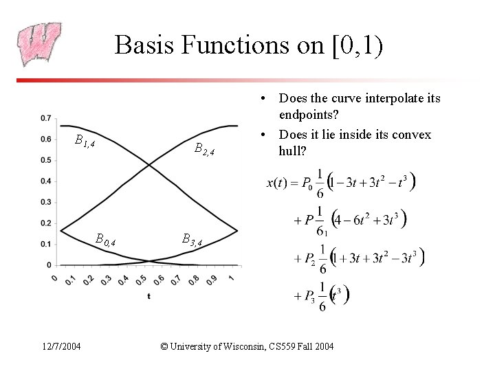
Basis Functions on [0, 1) B 1, 4 B 2, 4 B 0, 4 12/7/2004 • Does the curve interpolate its endpoints? • Does it lie inside its convex hull? B 3, 4 © University of Wisconsin, CS 559 Fall 2004

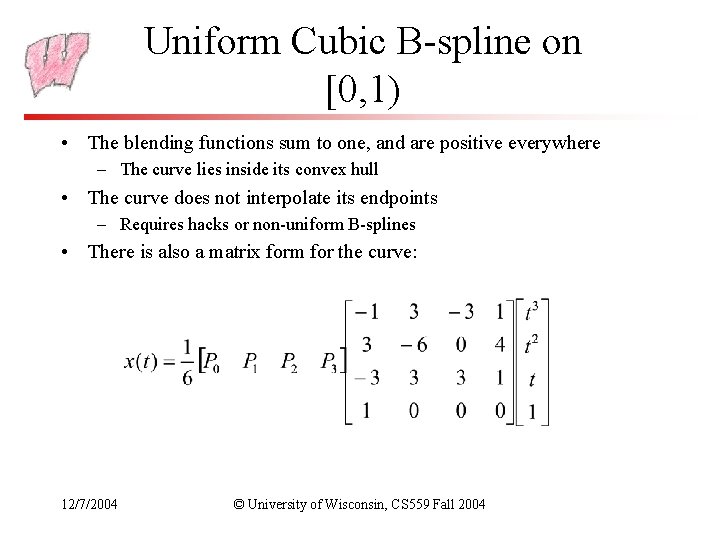
Uniform Cubic B-spline on [0, 1) • The blending functions sum to one, and are positive everywhere – The curve lies inside its convex hull • The curve does not interpolate its endpoints – Requires hacks or non-uniform B-splines • There is also a matrix form for the curve: 12/7/2004 © University of Wisconsin, CS 559 Fall 2004

Demo 12/7/2004 © University of Wisconsin, CS 559 Fall 2004

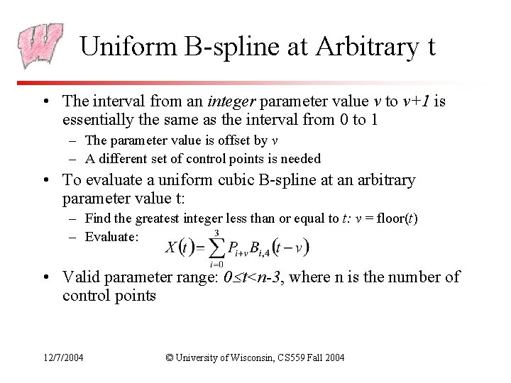
Uniform B-spline at Arbitrary t • The interval from an integer parameter value v to v+1 is essentially the same as the interval from 0 to 1 – The parameter value is offset by v – A different set of control points is needed • To evaluate a uniform cubic B-spline at an arbitrary parameter value t: – Find the greatest integer less than or equal to t: v = floor(t) – Evaluate: • Valid parameter range: 0 t<n-3, where n is the number of control points 12/7/2004 © University of Wisconsin, CS 559 Fall 2004

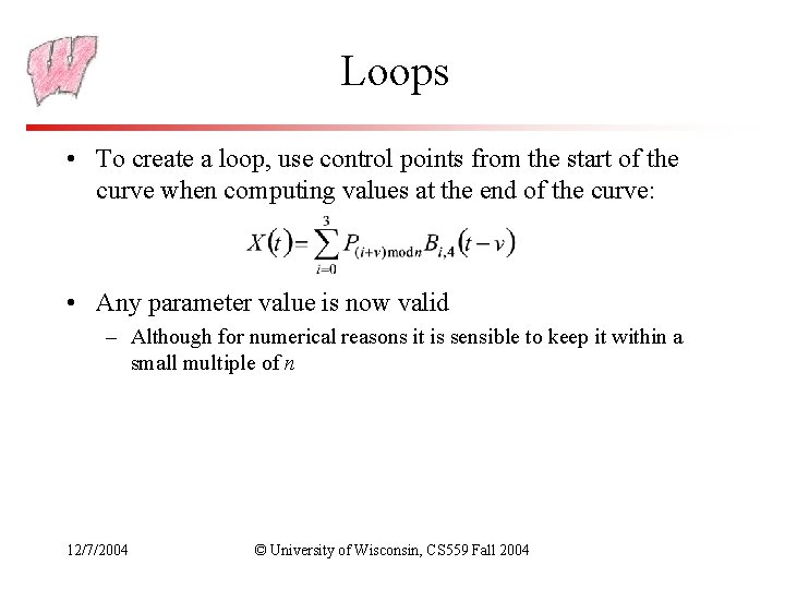
Loops • To create a loop, use control points from the start of the curve when computing values at the end of the curve: • Any parameter value is now valid – Although for numerical reasons it is sensible to keep it within a small multiple of n 12/7/2004 © University of Wisconsin, CS 559 Fall 2004

Demo 12/7/2004 © University of Wisconsin, CS 559 Fall 2004

B-splines and Interpolation, Continuity • Uniform B-splines do not interpolate control points, unless: – You repeat a control point three times – But then all derivatives also vanish (=0) at that point – To do interpolation with non-zero derivatives you must use non-uniform Bsplines with repeated knots • To align tangents, use double control vertices – Then tangent aligns similar to Bezier curve • Uniform B-splines are automatically C 2 – All the blending functions are C 2, so sum of blending functions is C 2 – Provides an alternate way to define blending functions – To reduce continuity, must use non-uniform B-splines with repeated knots 12/7/2004 © University of Wisconsin, CS 559 Fall 2004

Rendering B-splines • Same basic options as for Bezier curves – Evaluate at a set of parameter values and join with lines • Hard to know where to evaluate, and how pts to use – Use a subdivision rule to break the curve into small pieces, and then join control points • What is the subdivision rule for B-splines? • Instead of subdivision, view splitting as refinement: – Inserting additional control points, and knots, between the existing points – Useful not just for rendering - also a user interface tool – Defined for uniform and non-uniform B-splines by the Oslo algorithm 12/7/2004 © University of Wisconsin, CS 559 Fall 2004

Non-Uniform B-Splines • Uniform B-splines are a special case of B-splines – Each blending function is the same – A blending functions starts at t=-3, t=-2, t=-1, … – Each blending function is non-zero for 4 units of the parameter (if cubic) • Non-uniform B-splines – Blending functions not all the same – Blending functions can star or stop anywhere – Fine control of continuity, without vanishing derivatives • A deep investigation of B-splines is beyond the scope of this class 12/7/2004 © University of Wisconsin, CS 559 Fall 2004

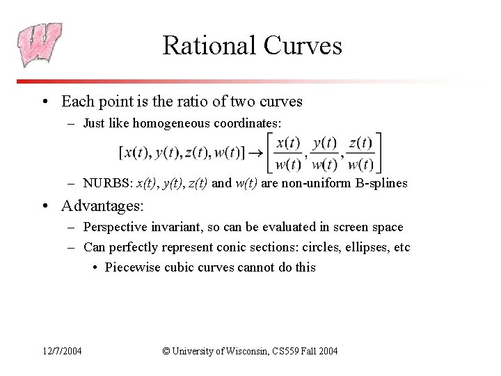
Rational Curves • Each point is the ratio of two curves – Just like homogeneous coordinates: – NURBS: x(t), y(t), z(t) and w(t) are non-uniform B-splines • Advantages: – Perspective invariant, so can be evaluated in screen space – Can perfectly represent conic sections: circles, ellipses, etc • Piecewise cubic curves cannot do this 12/7/2004 © University of Wisconsin, CS 559 Fall 2004

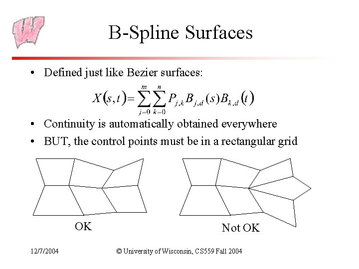
B-Spline Surfaces • Defined just like Bezier surfaces: • Continuity is automatically obtained everywhere • BUT, the control points must be in a rectangular grid OK 12/7/2004 Not OK © University of Wisconsin, CS 559 Fall 2004

How to Choose a Spline • Hermite curves are good for single segments where you know the parametric derivative or want easy control of it • Bezier curves are good for single segments or patches where a user controls the points • B-splines are good for large continuous curves and surfaces • NURBS are the most general, and are good when that generality is useful, or when conic sections must be accurately represented (CAD) 12/7/2004 © University of Wisconsin, CS 559 Fall 2004