Last Time Many many modeling techniques Polygon meshes

Last Time • Many, many modeling techniques – – – – Polygon meshes Parametric instancing Hierarchical modeling Constructive Solid Geometry Sweep Objects Octrees Blobs and Metaballs and other such things Production rules 04/16/02 (c) 2002, University of Wisconsin, CS 559

Today • Parametric curves – Hermite curves – Bezier curves • Midterms available in class 04/16/02 (c) 2002, University of Wisconsin, CS 559

Shortcomings So Far • The representations we have looked at so far have various failings: – – – Meshes are large, difficult to edit, require normal approximations, … Parametric instancing has a limited domain of shapes CSG is difficult to render and limited in range of shapes Implicit models are difficult to control and render Production rules work in highly limited domains • Parametric curves and surfaces address many of these issues – More general than parametric instancing – Easier to control than meshes and implicit models 04/16/02 (c) 2002, University of Wisconsin, CS 559

Why Parametric Curves? • Parametric curves are intended to provide the generality of polygon meshes but with fewer parameters for smooth surfaces – Polygon meshes have as many parameters as there are vertices (at least) • Fewer parameters makes it faster to create a curve, and easier to edit an existing curve • Normal fields can be properly defined everywhere • Parametric curves are easier to animate than polygon meshes 04/16/02 (c) 2002, University of Wisconsin, CS 559

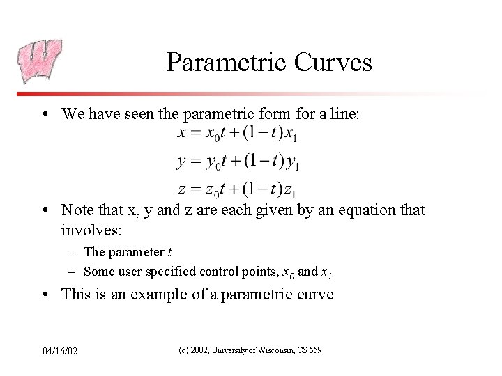
Parametric Curves • We have seen the parametric form for a line: • Note that x, y and z are each given by an equation that involves: – The parameter t – Some user specified control points, x 0 and x 1 • This is an example of a parametric curve 04/16/02 (c) 2002, University of Wisconsin, CS 559

Hermite Spline • A spline is a parametric curve defined by control points – The term spline dates from engineering drawing, where a spline was a piece of flexible wood used to draw smooth curves – The control points are adjusted by the user to control the shape of the curve • A Hermite spline is a curve for which the user provides: – The endpoints of the curve – The parametric derivatives of the curve at the endpoints • The parametric derivatives are dx/dt, dy/dt, dz/dt – That is enough to define a cubic Hermite spline, more derivatives are required for higher order curves 04/16/02 (c) 2002, University of Wisconsin, CS 559

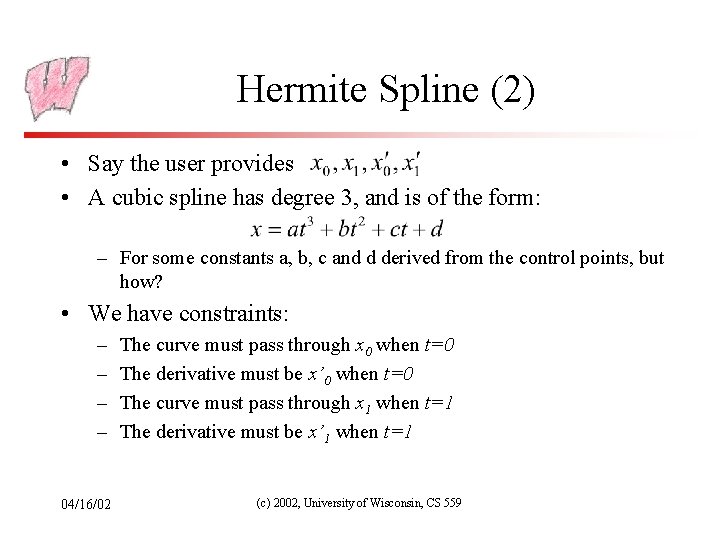
Hermite Spline (2) • Say the user provides • A cubic spline has degree 3, and is of the form: – For some constants a, b, c and d derived from the control points, but how? • We have constraints: – – 04/16/02 The curve must pass through x 0 when t=0 The derivative must be x’ 0 when t=0 The curve must pass through x 1 when t=1 The derivative must be x’ 1 when t=1 (c) 2002, University of Wisconsin, CS 559

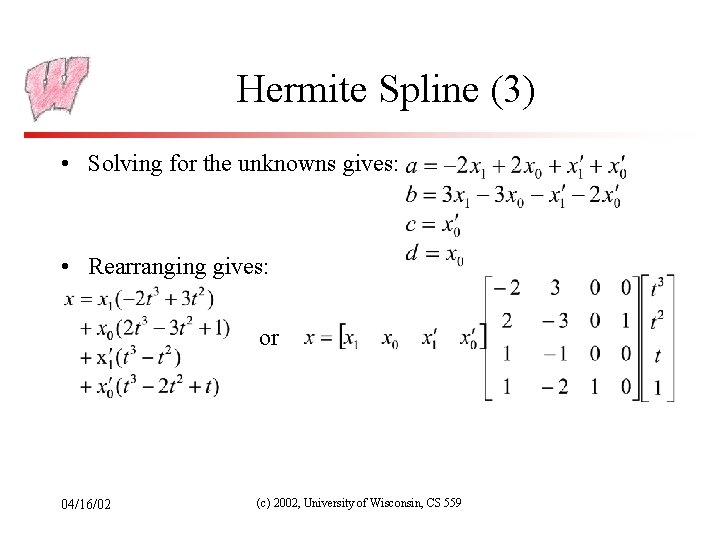
Hermite Spline (3) • Solving for the unknowns gives: • Rearranging gives: or 04/16/02 (c) 2002, University of Wisconsin, CS 559

Basis Functions • A point on a Hermite curve is obtained by multiplying each control point by some function and summing • The functions are called basis functions 04/16/02 (c) 2002, University of Wisconsin, CS 559

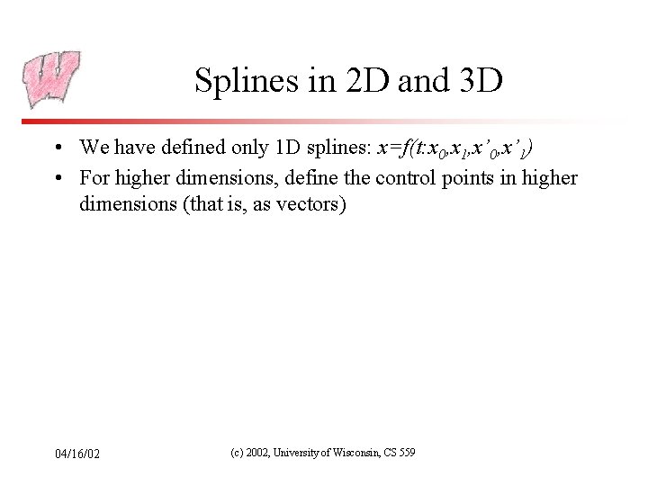
Splines in 2 D and 3 D • We have defined only 1 D splines: x=f(t: x 0, x 1, x’ 0, x’ 1) • For higher dimensions, define the control points in higher dimensions (that is, as vectors) 04/16/02 (c) 2002, University of Wisconsin, CS 559

Bezier Curves (1) • Different choices of basis functions give different curves – Choice of basis determines how the control points influence the curve – In Hermite case, two control points define endpoints, and two more define parametric derivatives • For Bezier curves, two control points define endpoints, and two control the tangents at the endpoints in a geometric way 04/16/02 (c) 2002, University of Wisconsin, CS 559

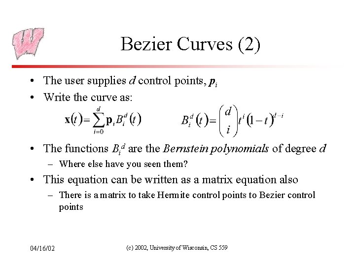
Bezier Curves (2) • The user supplies d control points, pi • Write the curve as: • The functions Bid are the Bernstein polynomials of degree d – Where else have you seen them? • This equation can be written as a matrix equation also – There is a matrix to take Hermite control points to Bezier control points 04/16/02 (c) 2002, University of Wisconsin, CS 559

Bezier Basis Functions for d=3 04/16/02 (c) 2002, University of Wisconsin, CS 559

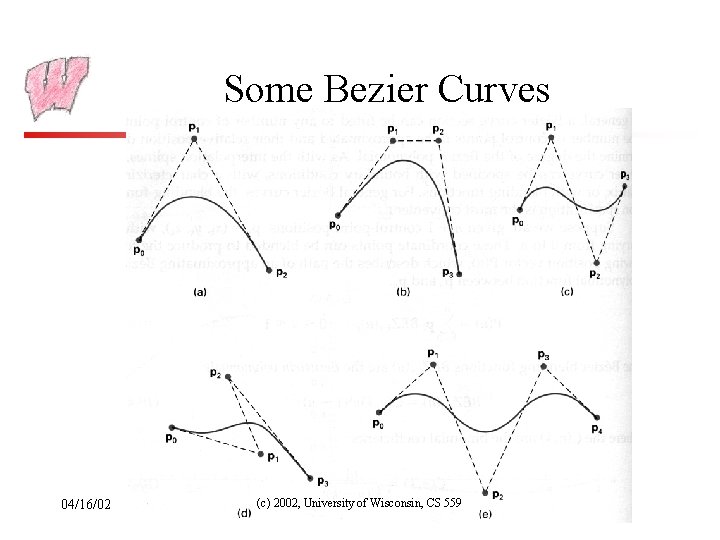
Some Bezier Curves 04/16/02 (c) 2002, University of Wisconsin, CS 559

Bezier Curve Properties • The first and last control points are interpolated • The tangent to the curve at the first control point is along the line joining the first and second control points • The tangent at the last control point is along the line joining the second last and last control points • The curve lies entirely within the convex hull of its control points – The Bernstein polynomials (the basis functions) sum to 1 and are everywhere positive • They can be rendered in many ways – E. g. : Convert to line segments with a subdivision algorithm 04/16/02 (c) 2002, University of Wisconsin, CS 559

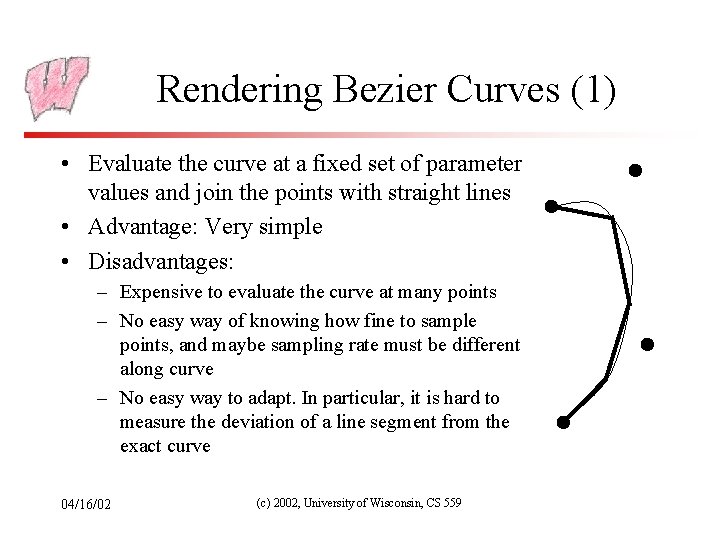
Rendering Bezier Curves (1) • Evaluate the curve at a fixed set of parameter values and join the points with straight lines • Advantage: Very simple • Disadvantages: – Expensive to evaluate the curve at many points – No easy way of knowing how fine to sample points, and maybe sampling rate must be different along curve – No easy way to adapt. In particular, it is hard to measure the deviation of a line segment from the exact curve 04/16/02 (c) 2002, University of Wisconsin, CS 559

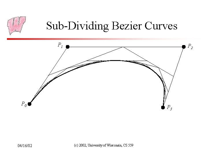
Rendering Bezier Curves (2) • Recall that a Bezier curve lies entirely within the convex hull of its control vertices • If the control vertices are nearly collinear, then the convex hull is a good approximation to the curve • Also, a cubic Bezier curve can be broken into two shorter cubic Bezier curves that exactly cover the original curve • This suggests a rendering algorithm: – Keep breaking the curve into sub-curves – Stop when the control points of each sub-curve are nearly collinear – Draw the control polygon - the polygon formed by the control points 04/16/02 (c) 2002, University of Wisconsin, CS 559

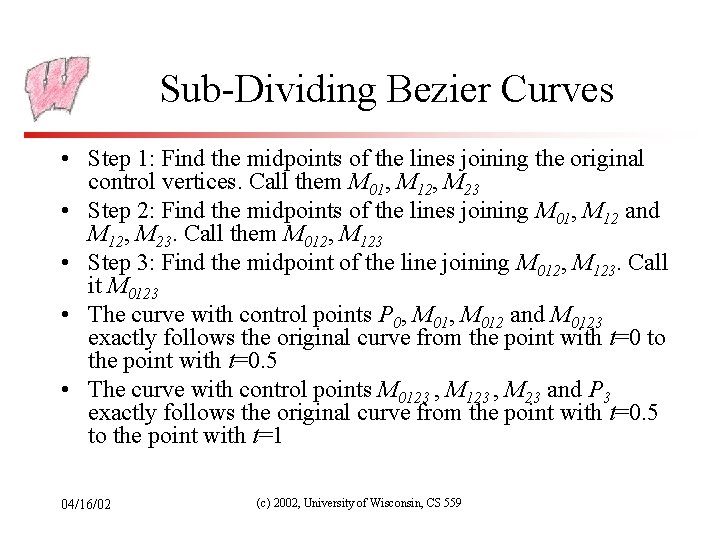
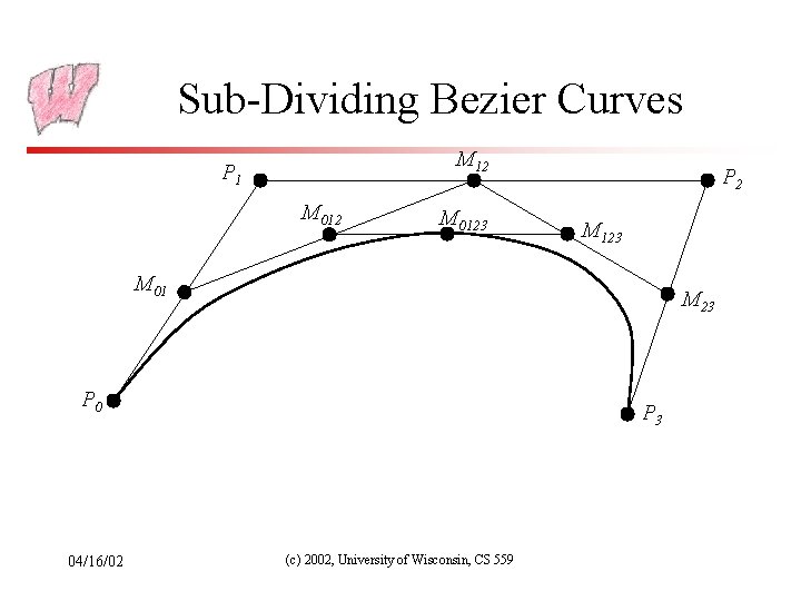
Sub-Dividing Bezier Curves • Step 1: Find the midpoints of the lines joining the original control vertices. Call them M 01, M 12, M 23 • Step 2: Find the midpoints of the lines joining M 01, M 12 and M 12, M 23. Call them M 012, M 123 • Step 3: Find the midpoint of the line joining M 012, M 123. Call it M 0123 • The curve with control points P 0, M 012 and M 0123 exactly follows the original curve from the point with t=0 to the point with t=0. 5 • The curve with control points M 0123 , M 23 and P 3 exactly follows the original curve from the point with t=0. 5 to the point with t=1 04/16/02 (c) 2002, University of Wisconsin, CS 559

Sub-Dividing Bezier Curves M 12 P 1 M 0123 P 2 M 123 M 01 M 23 P 0 04/16/02 P 3 (c) 2002, University of Wisconsin, CS 559

Sub-Dividing Bezier Curves P 1 P 2 P 0 04/16/02 P 3 (c) 2002, University of Wisconsin, CS 559

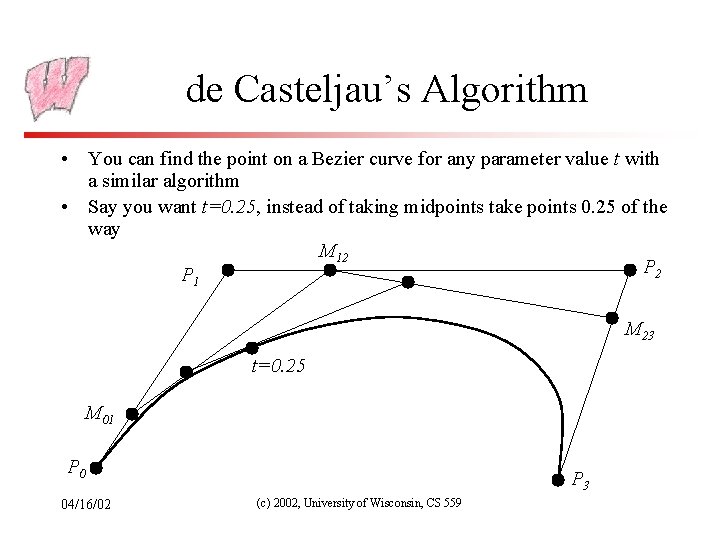
de Casteljau’s Algorithm • You can find the point on a Bezier curve for any parameter value t with a similar algorithm • Say you want t=0. 25, instead of taking midpoints take points 0. 25 of the way M 12 P 1 M 23 t=0. 25 M 01 P 0 04/16/02 P 3 (c) 2002, University of Wisconsin, CS 559

Invariance • Translational invariance means that translating the control points and then evaluating the curve is the same as evaluating and then translating the curve • Rotational invariance means that rotating the control points and then evaluating the curve is the same as evaluating and then rotating the curve • These properties are essential for parametric curves used in graphics • It is easy to prove that Bezier curves, Hermite curves and everything else we will study are translation and rotation invariant • Some forms of curves, rational splines, are also perspective invariant – Can do perspective transform of control points and then evaluate the curve 04/16/02 (c) 2002, University of Wisconsin, CS 559