
Last time Edge detection Convert a gray or



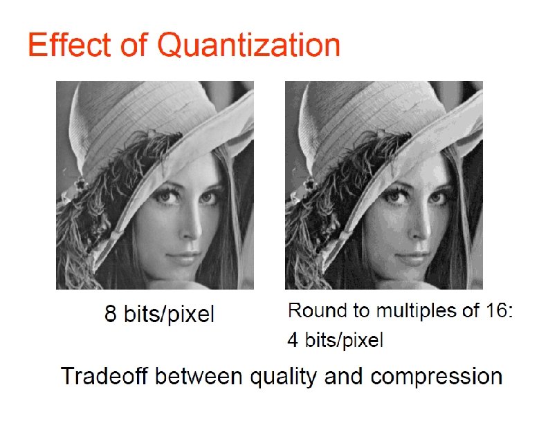
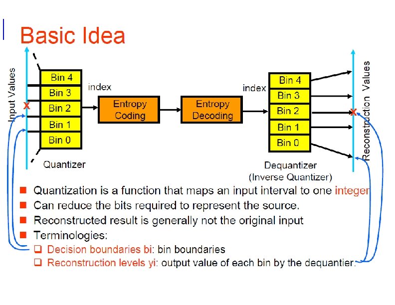
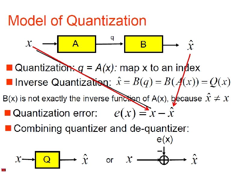
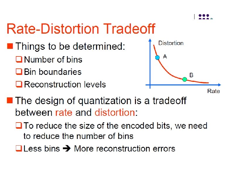




- Slides: 87
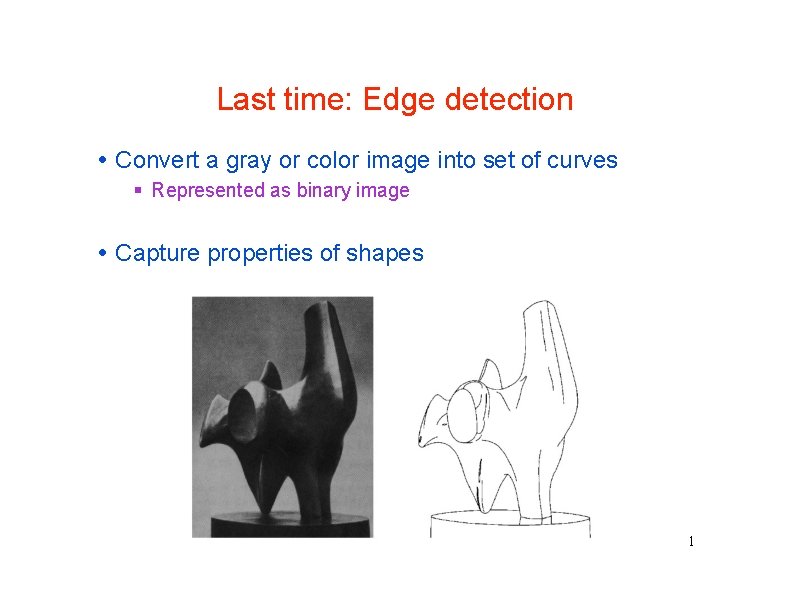
Last time: Edge detection Convert a gray or color image into set of curves Represented as binary image Capture properties of shapes 1
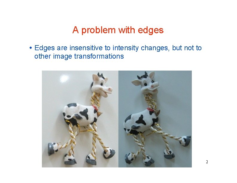
A problem with edges Edges are insensitive to intensity changes, but not to other image transformations 2
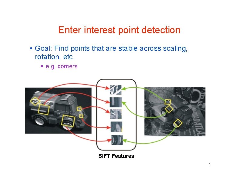
Enter interest point detection Goal: Find points that are stable across scaling, rotation, etc. e. g. corners SIFT Features 3
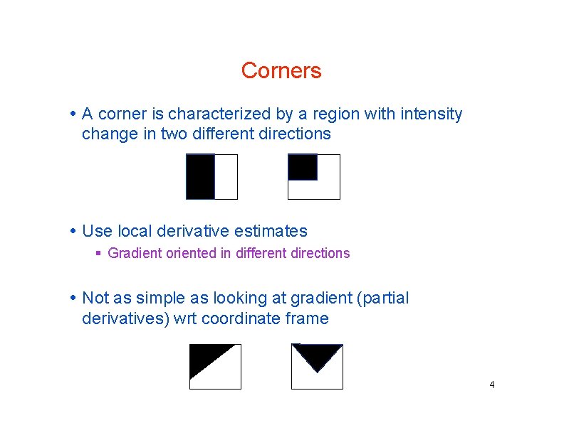
Corners A corner is characterized by a region with intensity change in two different directions Use local derivative estimates Gradient oriented in different directions Not as simple as looking at gradient (partial derivatives) wrt coordinate frame 4
Corner detection: the basic idea At a corner, shifting a window in any direction should give a large change in intensity “flat” region: no change in all directions “edge”: no change along the edge direction “corner”: significant change in all directions 5
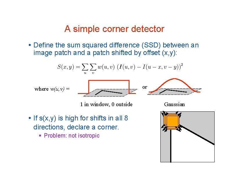
A simple corner detector Define the sum squared difference (SSD) between an image patch and a patch shifted by offset (x, y): or where w(u, v) = 1 in window, 0 outside If s(x, y) is high for shifts in all 8 directions, declare a corner. Problem: not isotropic Gaussian 7
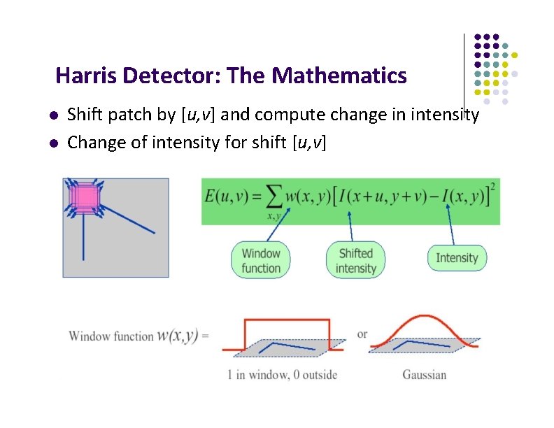
Harris Detector: The Mathematics Shift patch by [u, v] and compute change in intensity Change of intensity for shift [u, v]
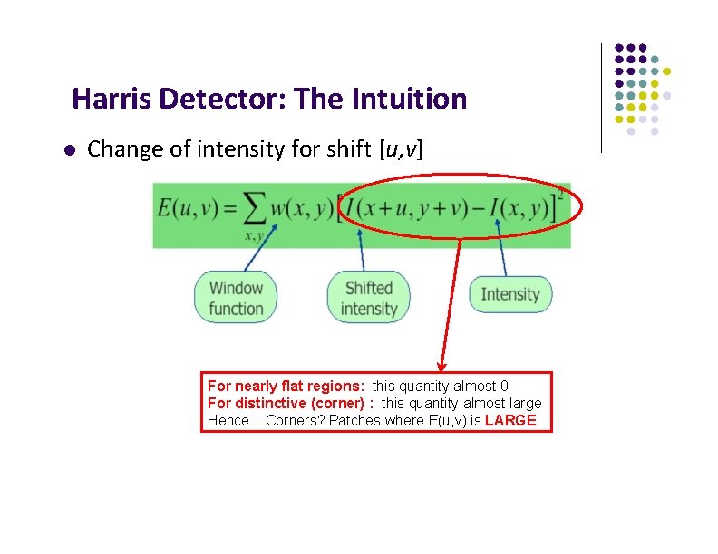
Harris Detector: The Intuition Change of intensity for shift [u, v] For nearly flat regions: this quantity almost 0 For distinctive (corner) : this quantity almost large Hence. . . Corners? Patches where E(u, v) is LARGE
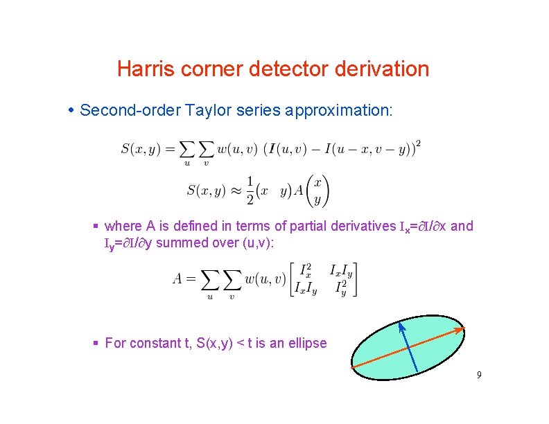
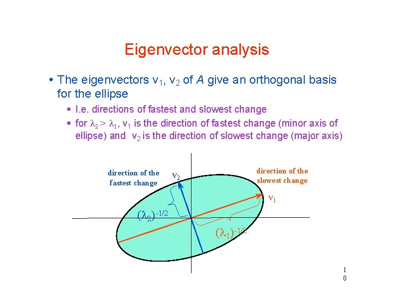
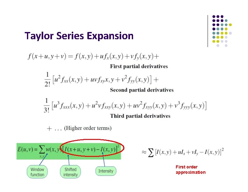
Harris corner detector derivation Second-order Taylor series approximation: where A is defined in terms of partial derivatives Ix= I/ x and Iy= I/ y summed over (u, v): For constant t, S(x, y) < t is an ellipse 9
Eigenvector analysis The eigenvectors v 1, v 2 of A give an orthogonal basis for the ellipse I. e. directions of fastest and slowest change for 2 > 1, v 1 is the direction of fastest change (minor axis of ellipse) and v 2 is the direction of slowest change (major axis) direction of the fastest change direction of the slowest change v 2 v 1 ( 2)-1/2 ( 1)-1/2 1 0
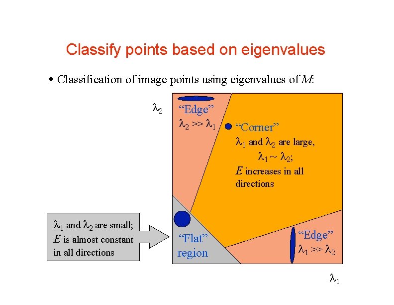
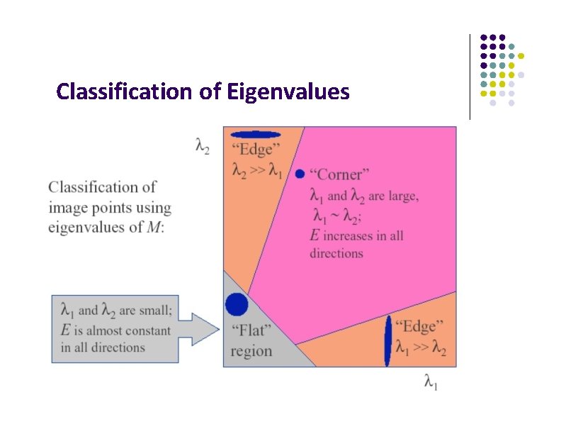
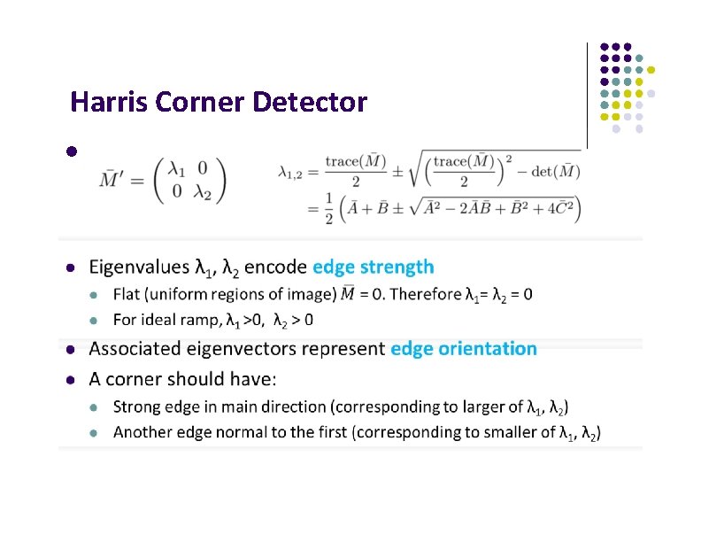
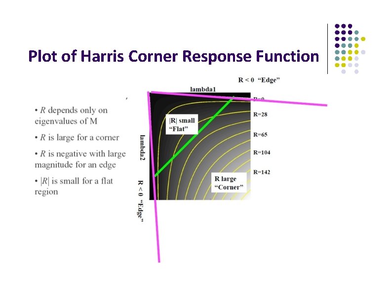
Classify points based on eigenvalues Classification of image points using eigenvalues of M: 2 “Edge” 2 >> 1 “Corner” 1 and 2 are large, 1 ~ 2; E increases in all directions 1 and 2 are small; E is almost constant in all directions “Flat” region “Edge” 1 >> 2 10 1
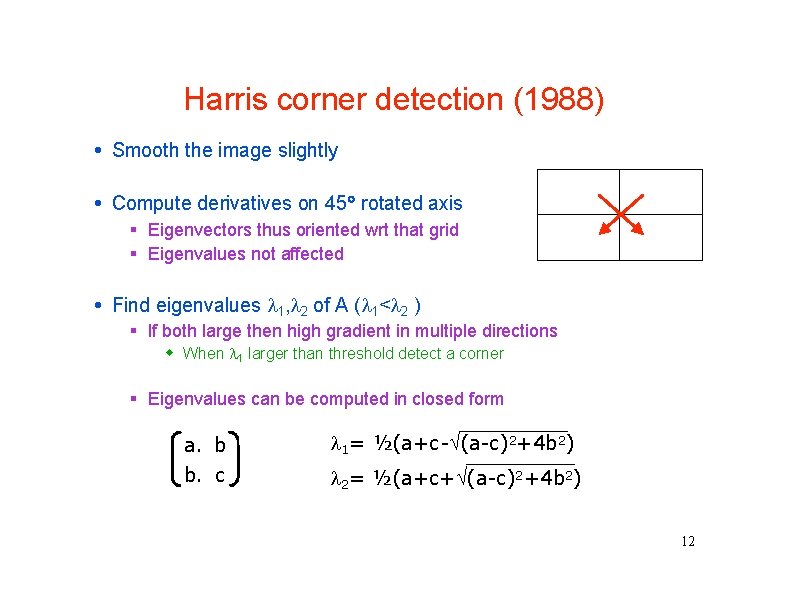
Harris corner detection (1988) Smooth the image slightly Compute derivatives on 45 rotated axis Eigenvectors thus oriented wrt that grid Eigenvalues not affected Find eigenvalues 1, 2 of A ( 1< 2 ) If both large then high gradient in multiple directions When 1 larger than threshold detect a corner Eigenvalues can be computed in closed form a. b b. c 1= ½(a+c- (a-c)2+4 b 2) 2= ½(a+c+ (a-c)2+4 b 2) 12
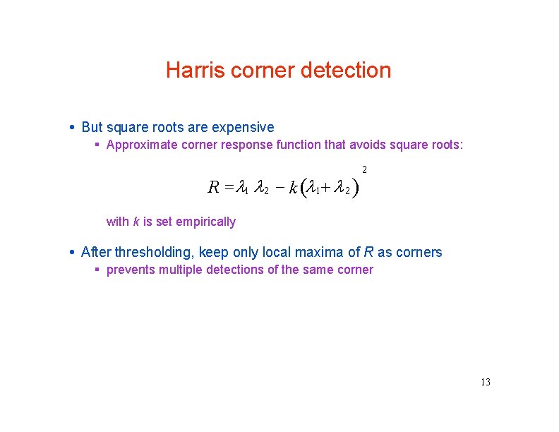
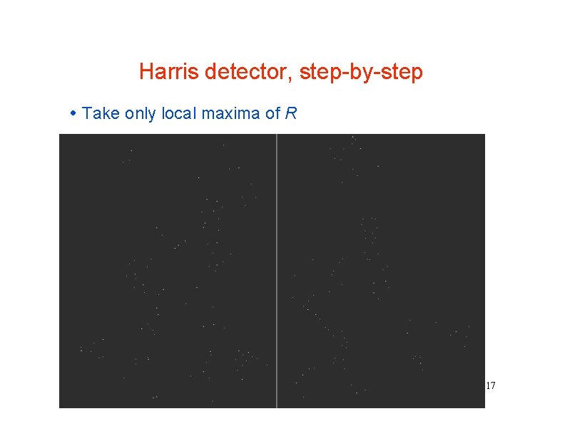
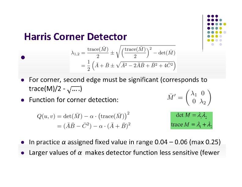
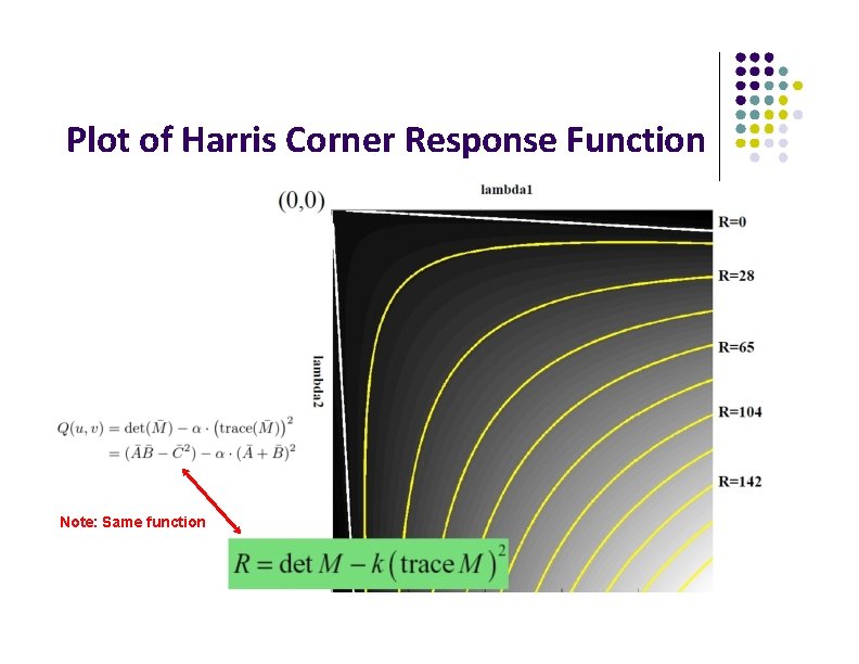
Harris corner detection But square roots are expensive Approximate corner response function that avoids square roots: R 1 2 k 1 2 2 with k is set empirically After thresholding, keep only local maxima of R as corners prevents multiple detections of the same corner 13
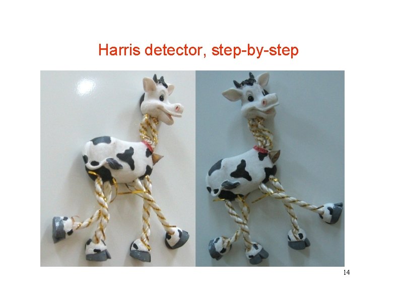
Harris detector, step-by-step 14
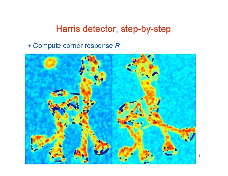
Harris detector, step-by-step Compute corner response R 15
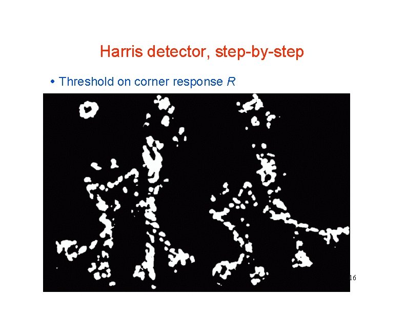
Harris detector, step-by-step Threshold on corner response R 16
Harris detector, step-by-step Take only local maxima of R 17
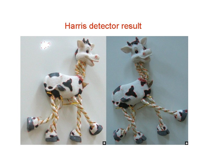
Harris detector result 18
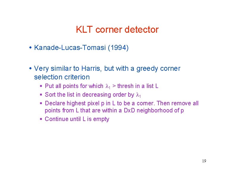
KLT corner detector Kanade-Lucas-Tomasi (1994) Very similar to Harris, but with a greedy corner selection criterion Put all points for which 1 > thresh in a list L Sort the list in decreasing order by 1 Declare highest pixel p in L to be a corner. Then remove all points from L that are within a Dx. D neighborhood of p Continue until L is empty 19
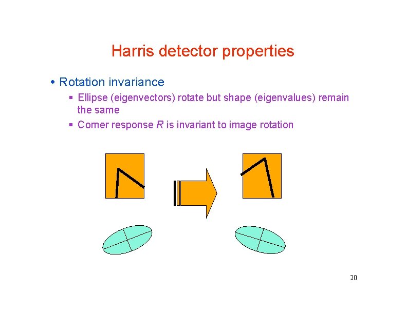
Harris detector properties Rotation invariance Ellipse (eigenvectors) rotate but shape (eigenvalues) remain the same Corner response R is invariant to image rotation 20
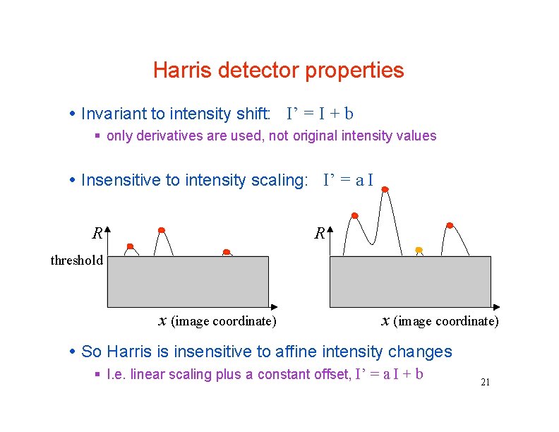
Harris detector properties Invariant to intensity shift: I’ = I + b only derivatives are used, not original intensity values Insensitive to intensity scaling: I’ = a I R R threshold x (image coordinate) So Harris is insensitive to affine intensity changes I. e. linear scaling plus a constant offset, I’ = a I + b 21
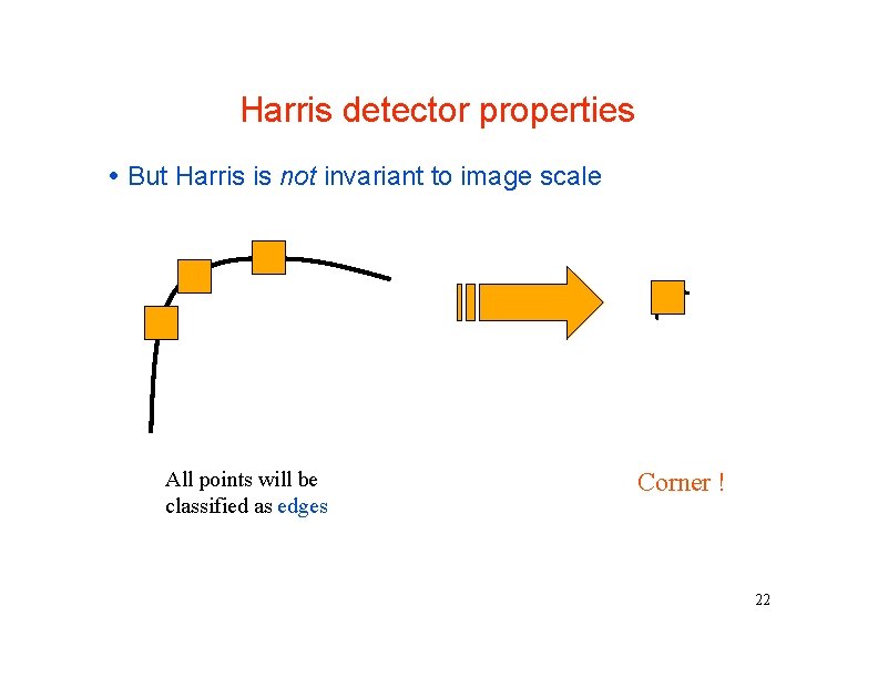
Harris detector properties But Harris is not invariant to image scale All points will be classified as edges Corner ! 22
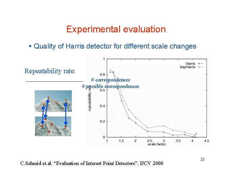
Experimental evaluation Quality of Harris detector for different scale changes Repeatability rate: # correspondences # possible correspondences C. Schmid et. al. “Evaluation of Interest Point Detectors”. IJCV 2000 23
Taylor Series Expansion First order approximation
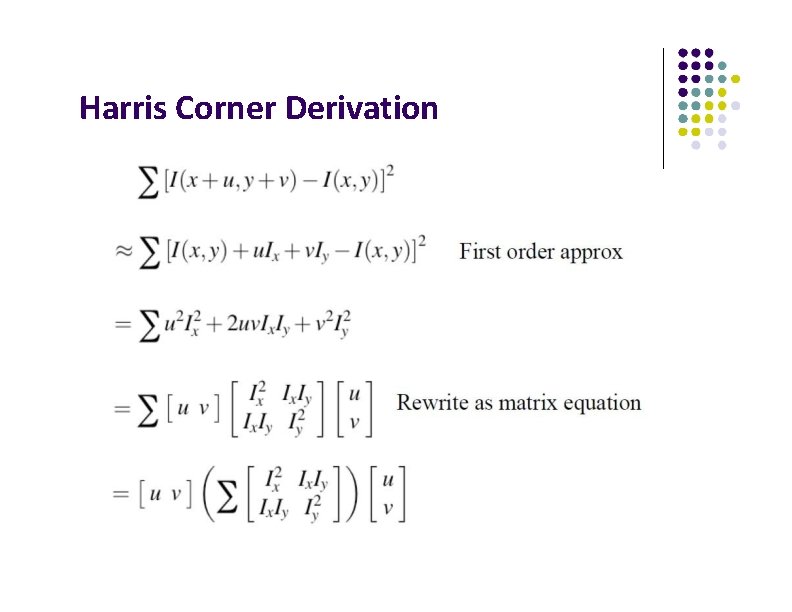
Harris Corner Derivation
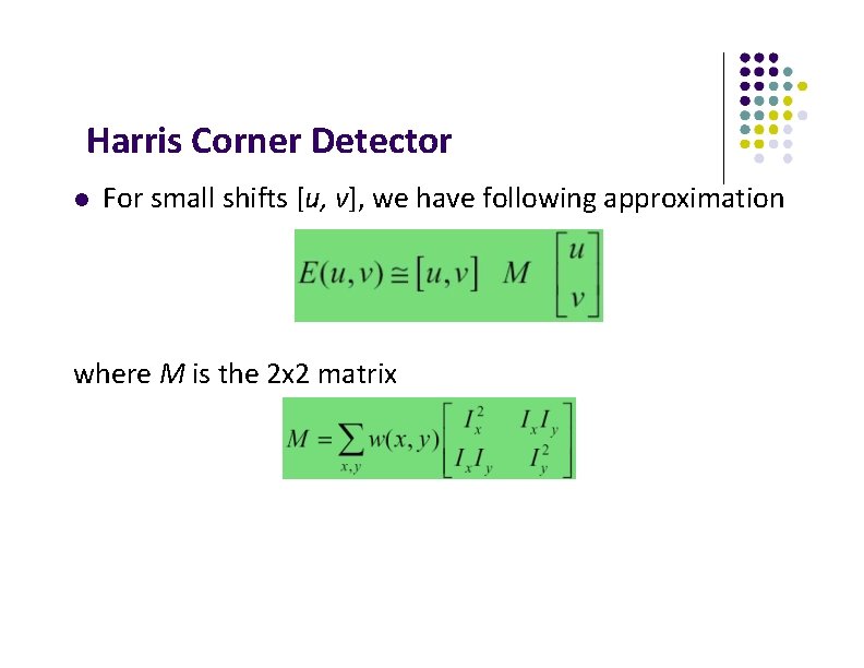
Harris Corner Detector For small shifts [u, v], we have following approximation where M is the 2 x 2 matrix
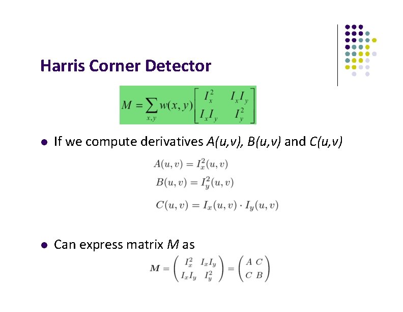
Harris Corner Detector If we compute derivatives A(u, v), B(u, v) and C(u, v) Can express matrix M as
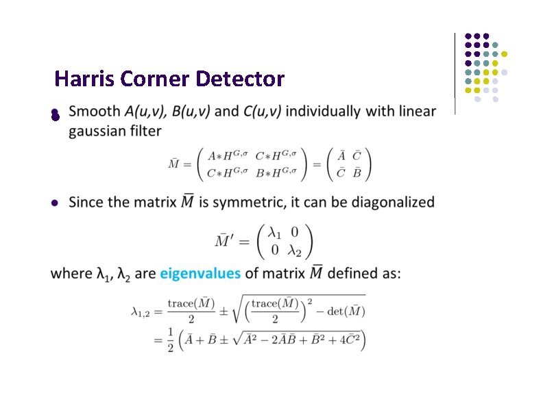
Harris Corner Detector
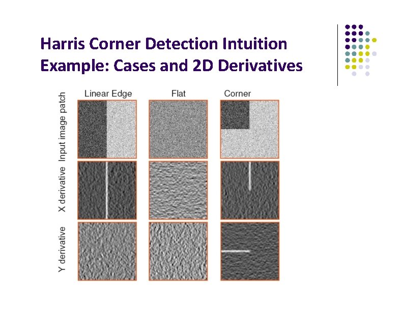
Harris Corner Detection Intuition Example: Cases and 2 D Derivatives
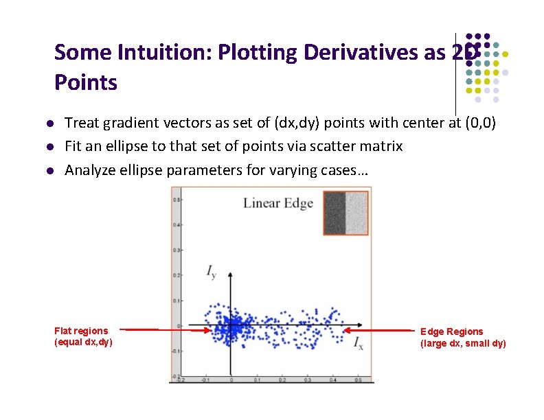
Some Intuition: Plotting Derivatives as 2 D Points Treat gradient vectors as set of (dx, dy) points with center at (0, 0) Fit an ellipse to that set of points via scatter matrix Analyze ellipse parameters for varying cases… Flat regions (equal dx, dy) Edge Regions (large dx, small dy)
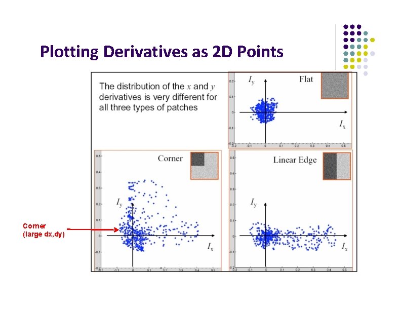
Plotting Derivatives as 2 D Points Corner (large dx, dy)
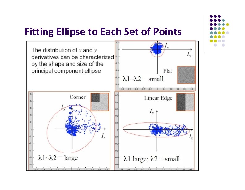
Fitting Ellipse to Each Set of Points
Classification of Eigenvalues
Harris Corner Detector
Harris Corner Detector
Plot of Harris Corner Response Function Note: Same function
Plot of Harris Corner Response Function
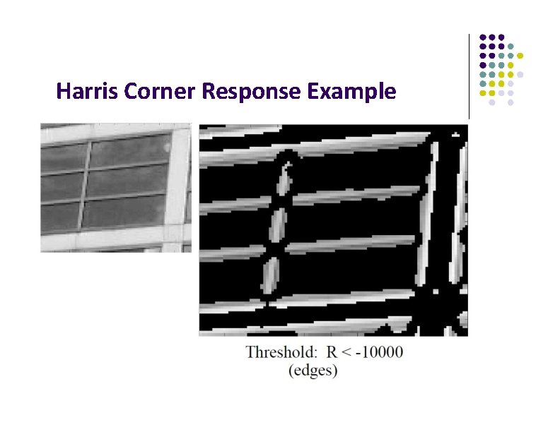
Harris Corner Response Example
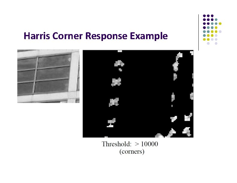
Harris Corner Response Example
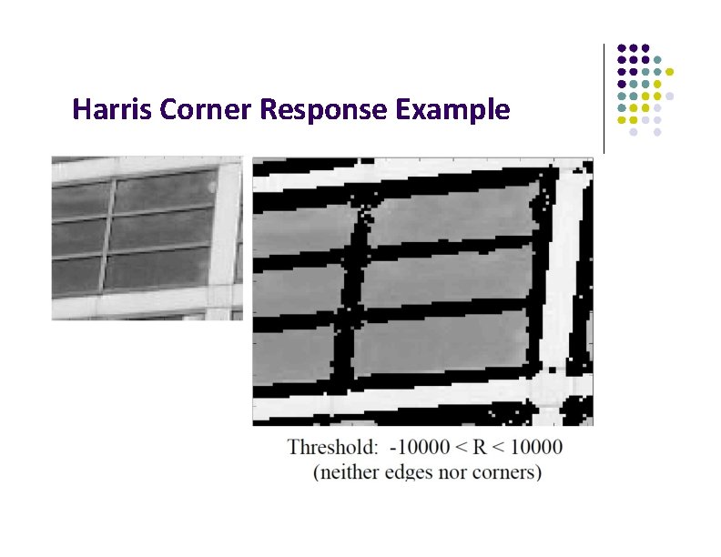
Harris Corner Response Example
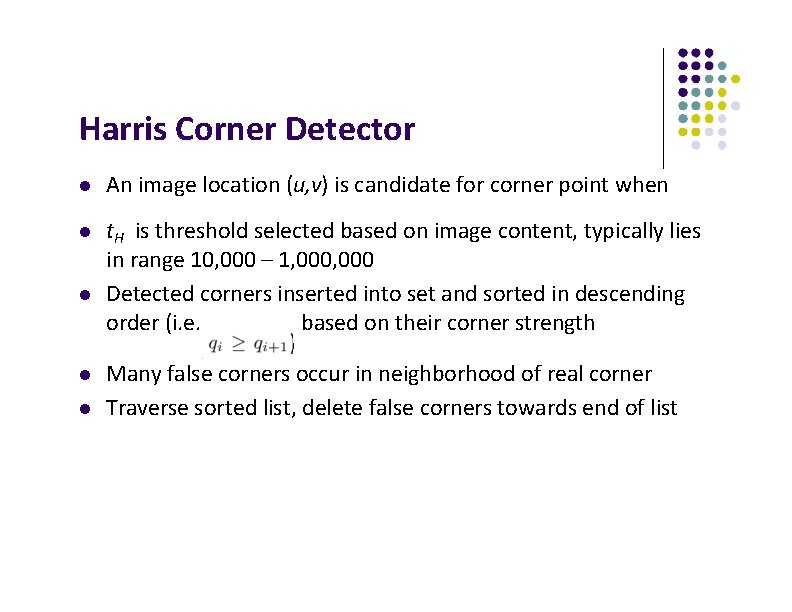
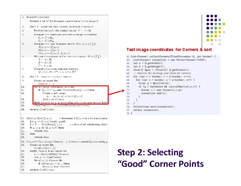
Harris Corner Detector An image location (u, v) is candidate for corner point when t. H is threshold selected based on image content, typically lies in range 10, 000 – 1, 000 Detected corners inserted into set and sorted in descending order (i. e. based on their corner strength ) Many false corners occur in neighborhood of real corner Traverse sorted list, delete false corners towards end of list
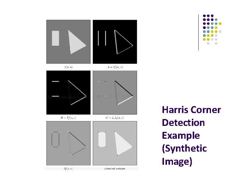
Harris Corner Detection Example (Synthetic Image)
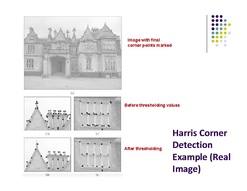
Image with final corner points marked Before thresholding values After thresholding Harris Corner Detection Example (Real Image)
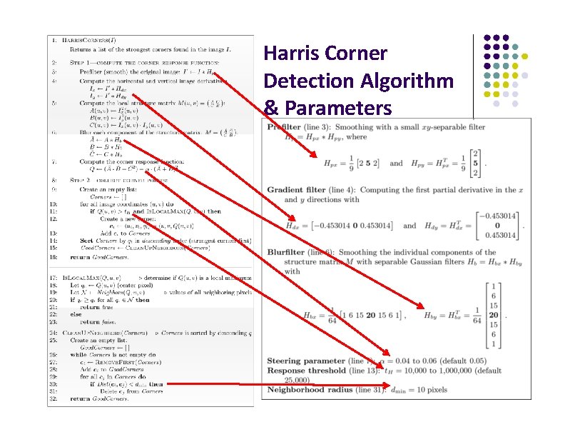
Harris Corner Detection Algorithm
Harris Corner Detection Algorithm & Parameters
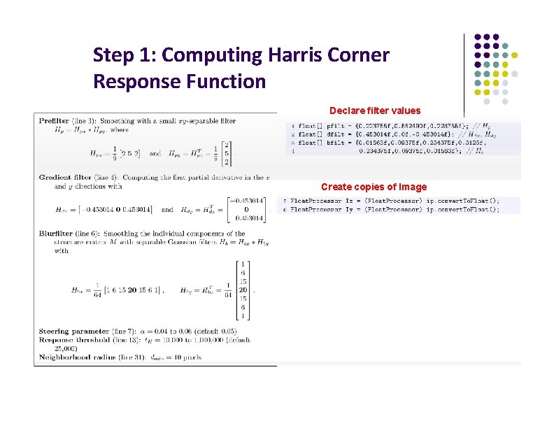
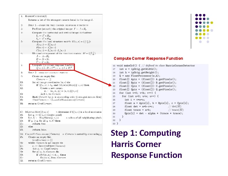
Step 1: Computing Harris Corner Response Function Declare filter values Create copies of Image
Apply pre-smoothing + gradient computation in one combined step Compute components A, B, C and smooth Step 1: Computing Harris Corner Response Function
Compute Corner Response Function Step 1: Computing Harris Corner Response Function
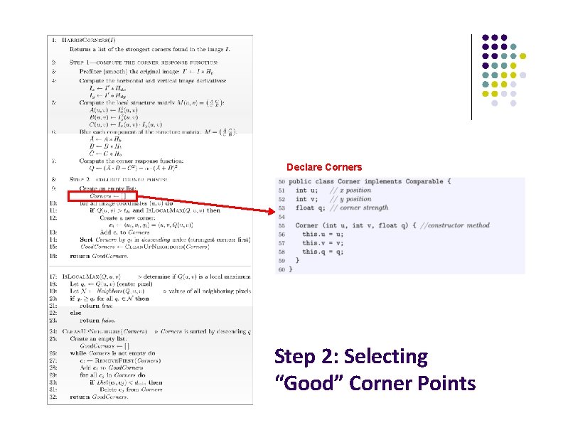
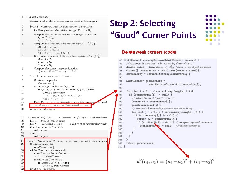
Declare Corners Step 2: Selecting “Good” Corner Points
Test image coordinates for Corners & sort Step 2: Selecting “Good” Corner Points
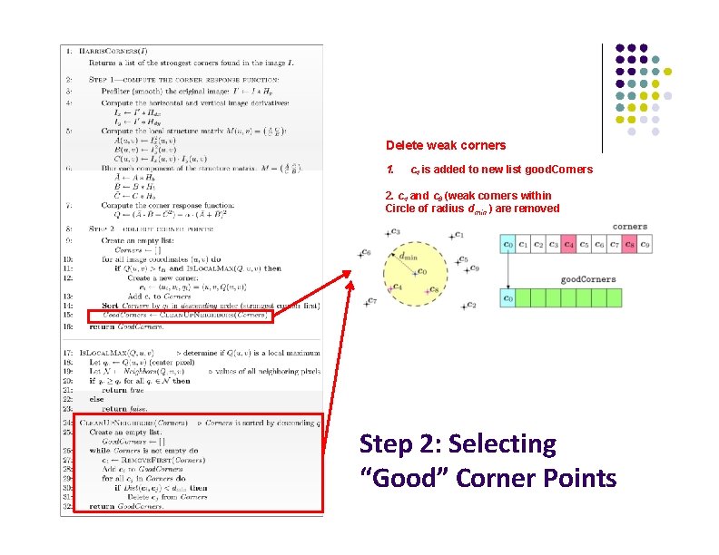
Delete weak corners 1. c 4 is added to new list good. Corners 2. c 4 and c 8 (weak corners within Circle of radius dmin ) are removed Step 2: Selecting “Good” Corner Points
Step 2: Selecting “Good” Corner Points Delete weak corners (code)
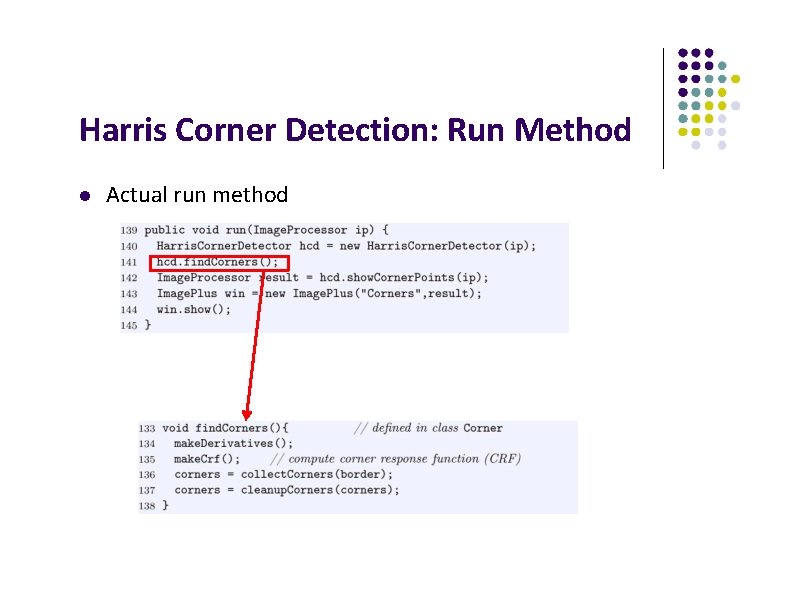
Harris Corner Detection: Run Method Actual run method
References Wilhelm Burger and Mark J. Burge, Digital Image Processing, Springer, 2008 Robert Collins, CSE 486 slides, Penn State University of Utah, CS 4640: Image Processing Basics, Spring 2012 Rutgers University, CS 334, Introduction to Imaging and Multimedia, Fall 2012 Gonzales and Woods, Digital Image Processing (3 rd edition), Prentice Hall
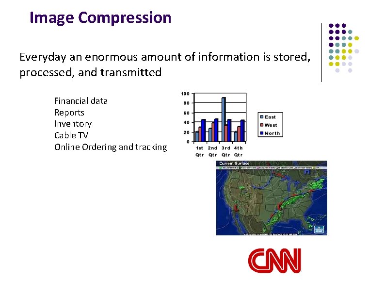
Image Compression Everyday an enormous amount of information is stored, processed, and transmitted Financial data Reports Inventory Cable TV Online Ordering and tracking
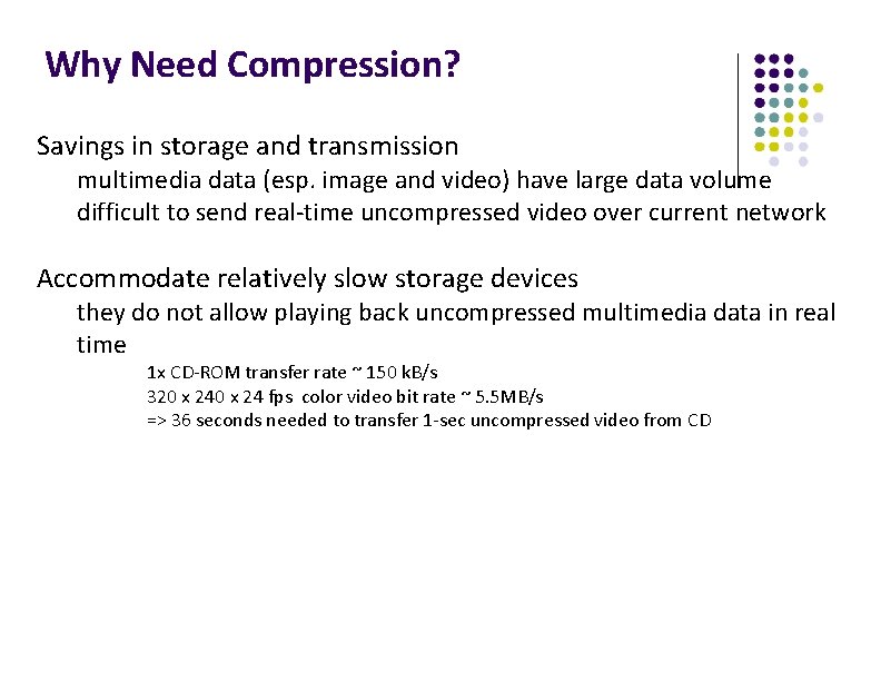
Why Need Compression? Savings in storage and transmission multimedia data (esp. image and video) have large data volume difficult to send real-time uncompressed video over current network Accommodate relatively slow storage devices they do not allow playing back uncompressed multimedia data in real time 1 x CD-ROM transfer rate ~ 150 k. B/s 320 x 24 fps color video bit rate ~ 5. 5 MB/s => 36 seconds needed to transfer 1 -sec uncompressed video from CD
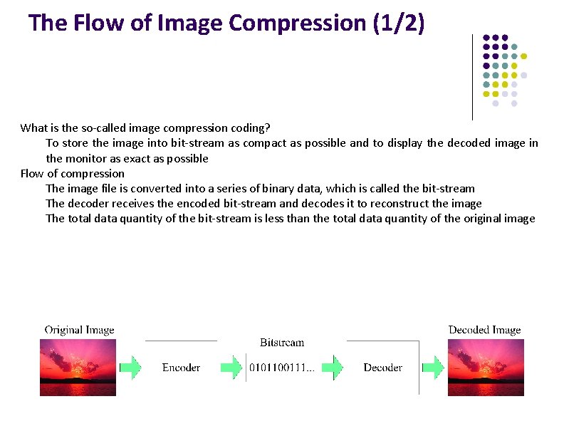
The Flow of Image Compression (1/2) What is the so-called image compression coding? To store the image into bit-stream as compact as possible and to display the decoded image in the monitor as exact as possible Flow of compression The image file is converted into a series of binary data, which is called the bit-stream The decoder receives the encoded bit-stream and decodes it to reconstruct the image The total data quantity of the bit-stream is less than the total data quantity of the original image
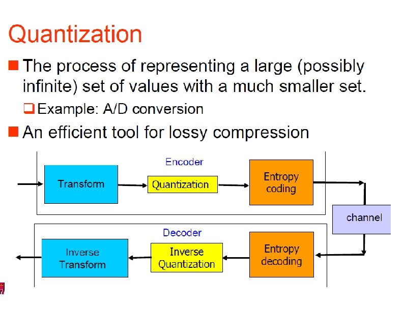
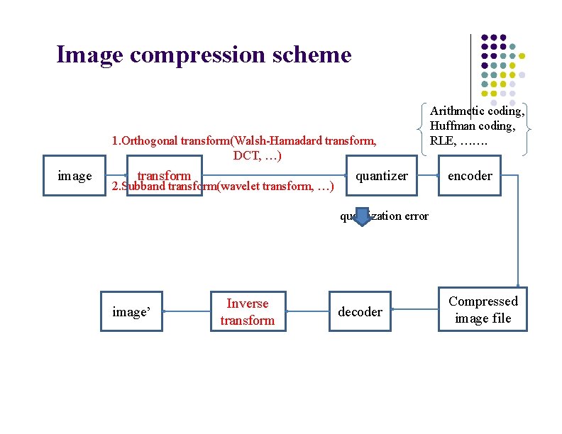
Image compression scheme 1. Orthogonal transform(Walsh-Hamadard transform, DCT, …) image transform 2. Subband transform(wavelet transform, …) quantizer Arithmetic coding, Huffman coding, RLE, ……. encoder quantization error image’ Inverse transform decoder Compressed image file
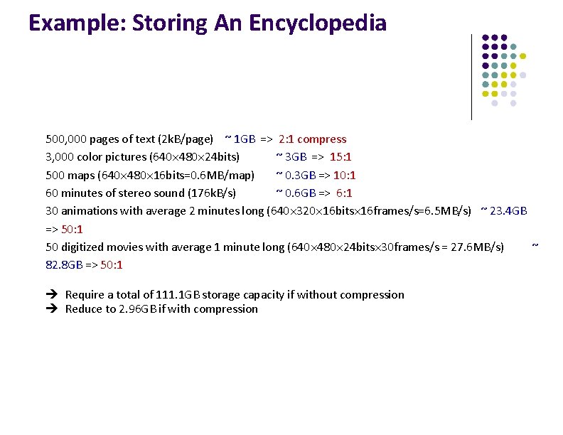
Example: Storing An Encyclopedia 500, 000 pages of text (2 k. B/page) ~ 1 GB => 2: 1 compress 3, 000 color pictures (640 480 24 bits) ~ 3 GB => 15: 1 500 maps (640 480 16 bits=0. 6 MB/map) ~ 0. 3 GB => 10: 1 60 minutes of stereo sound (176 k. B/s) ~ 0. 6 GB => 6: 1 30 animations with average 2 minutes long (640 320 16 bits 16 frames/s=6. 5 MB/s) ~ 23. 4 GB => 50: 1 50 digitized movies with average 1 minute long (640 480 24 bits 30 frames/s = 27. 6 MB/s) ~ 82. 8 GB => 50: 1 è Require a total of 111. 1 GB storage capacity if without compression è Reduce to 2. 96 GB if with compression
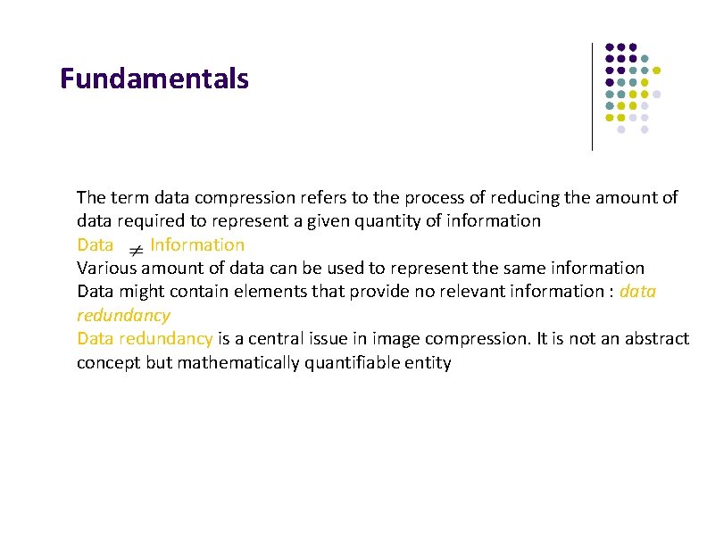
Fundamentals The term data compression refers to the process of reducing the amount of data required to represent a given quantity of information Data Information Various amount of data can be used to represent the same information Data might contain elements that provide no relevant information : data redundancy Data redundancy is a central issue in image compression. It is not an abstract concept but mathematically quantifiable entity
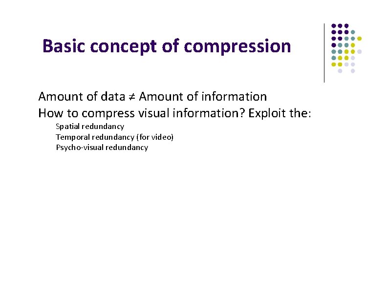
Basic concept of compression Amount of data ≠ Amount of information How to compress visual information? Exploit the: Spatial redundancy Temporal redundancy (for video) Psycho-visual redundancy
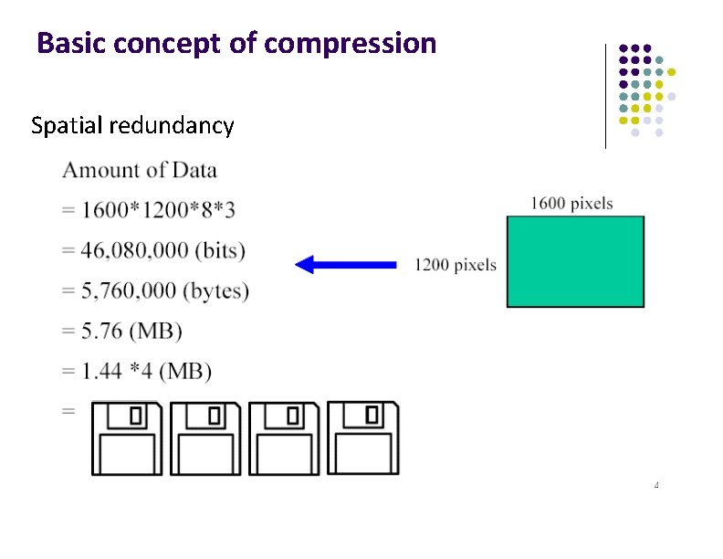
Basic concept of compression Spatial redundancy
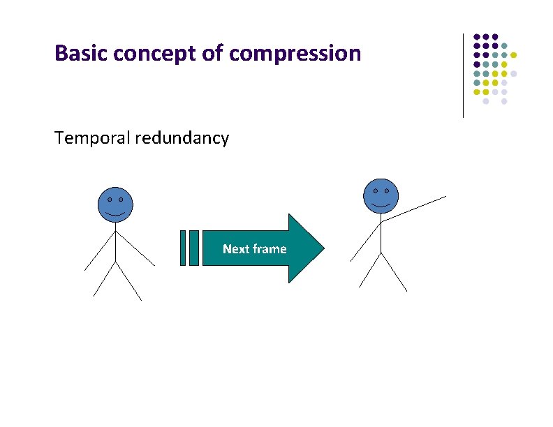
Basic concept of compression Temporal redundancy Next frame
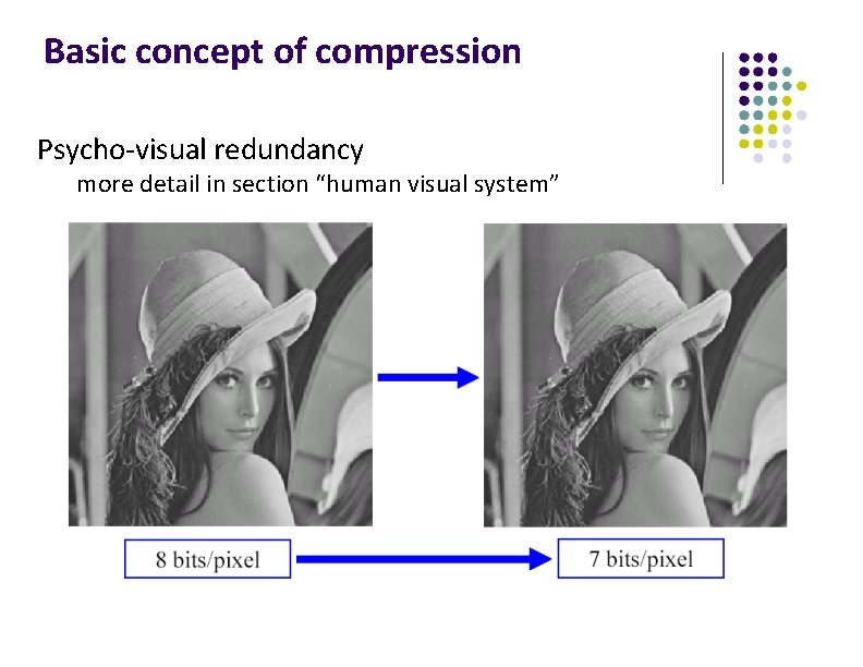
Basic concept of compression Psycho-visual redundancy more detail in section “human visual system”
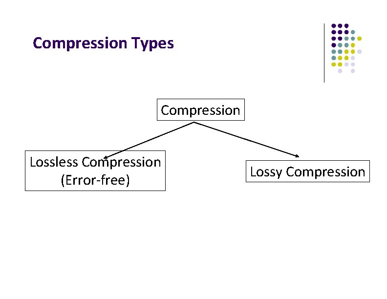
Compression Types Compression Lossless Compression (Error-free) Lossy Compression
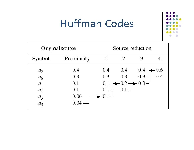
Huffman Codes
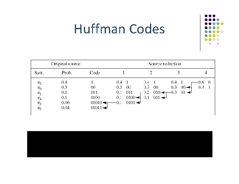
Huffman Codes
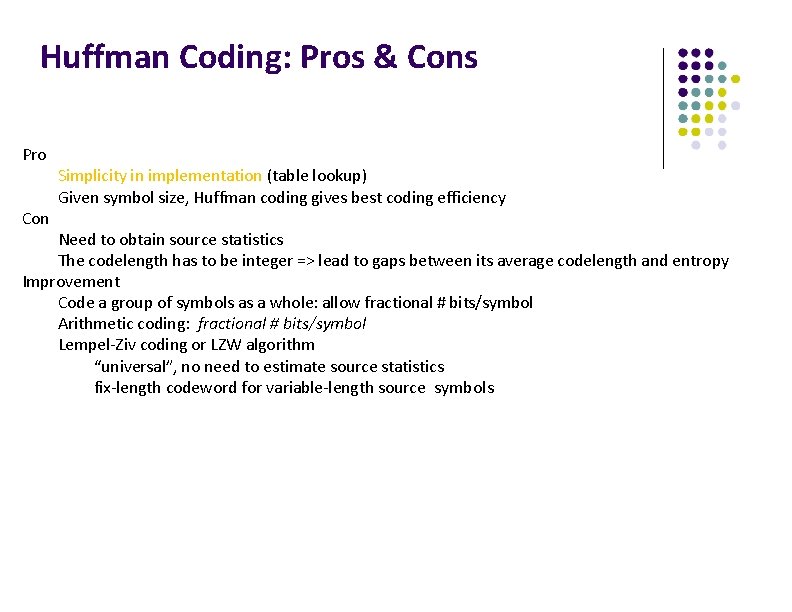
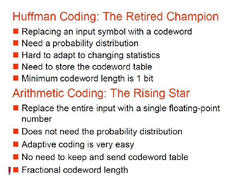
Huffman Coding: Pros & Cons Pro Con Simplicity in implementation (table lookup) Given symbol size, Huffman coding gives best coding efficiency Need to obtain source statistics The codelength has to be integer => lead to gaps between its average codelength and entropy Improvement Code a group of symbols as a whole: allow fractional # bits/symbol Arithmetic coding: fractional # bits/symbol Lempel-Ziv coding or LZW algorithm “universal”, no need to estimate source statistics fix-length codeword for variable-length source symbols