Last Lecture The radiusofgyration of a polymer Rg

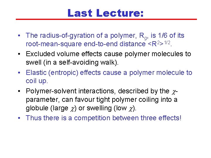
Last Lecture: • The radius-of-gyration of a polymer, Rg, is 1/6 of its root-mean-square end-to-end distance <R 2>1/2. • Excluded volume effects cause polymer molecules to swell (in a self-avoiding walk). • Elastic (entropic) effects cause a polymer molecule to coil up. • Polymer-solvent interactions, described by the cparameter, can favour tight polymer coiling into a globule (large c) or swelling (low c). • Thus there is a competition between three effects!

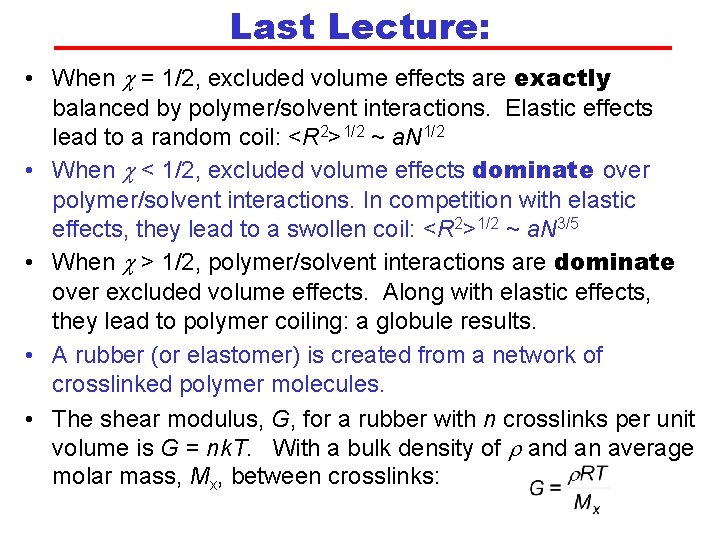
Last Lecture: • When c = 1/2, excluded volume effects are exactly balanced by polymer/solvent interactions. Elastic effects lead to a random coil: <R 2>1/2 ~ a. N 1/2 • When c < 1/2, excluded volume effects dominate over polymer/solvent interactions. In competition with elastic effects, they lead to a swollen coil: <R 2>1/2 ~ a. N 3/5 • When c > 1/2, polymer/solvent interactions are dominate over excluded volume effects. Along with elastic effects, they lead to polymer coiling: a globule results. • A rubber (or elastomer) is created from a network of crosslinked polymer molecules. • The shear modulus, G, for a rubber with n crosslinks per unit volume is G = nk. T. With a bulk density of r and an average molar mass, Mx, between crosslinks:

3 SMS Polymer Reptation, Viscosity and Diffusion 20 March, 2007 Lecture 10 See Jones’ Soft Condensed Matter, Chapt. 5

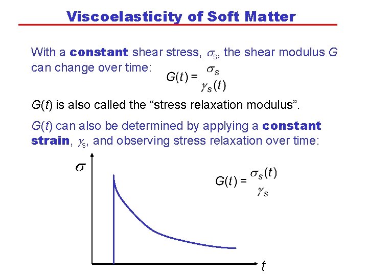
Viscoelasticity of Soft Matter With a constant shear stress, the shear modulus G can change over time: G(t) is also called the “stress relaxation modulus”. G(t) can also be determined by applying a constant strain, gs, and observing stress relaxation over time: s t

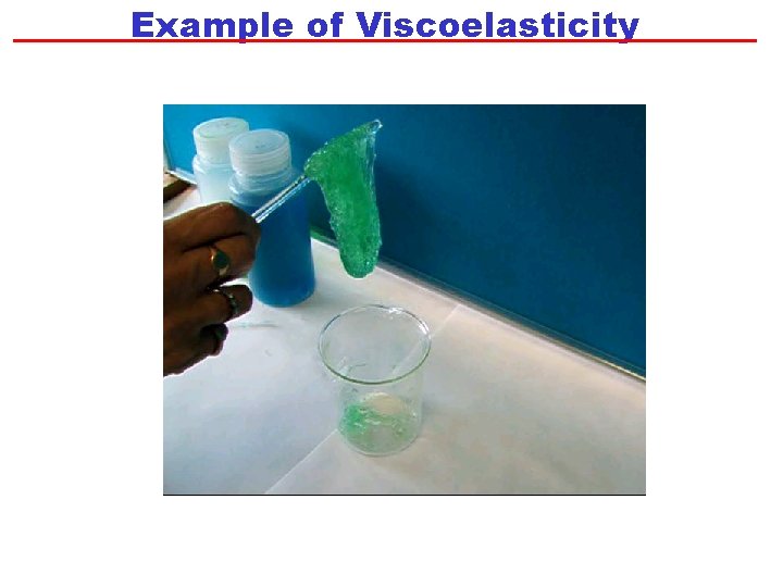
Example of Viscoelasticity

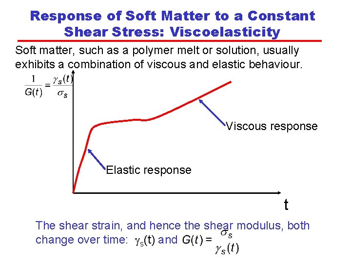
Response of Soft Matter to a Constant Shear Stress: Viscoelasticity Soft matter, such as a polymer melt or solution, usually exhibits a combination of viscous and elastic behaviour. Viscous response Elastic response t The shear strain, and hence the shear modulus, both change over time: gs(t) and

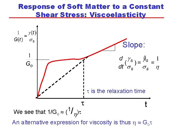
Response of Soft Matter to a Constant Shear Stress: Viscoelasticity Slope: t is the relaxation time t We see that 1/Go (1/h)t t An alternative expression for viscosity is thus h Got

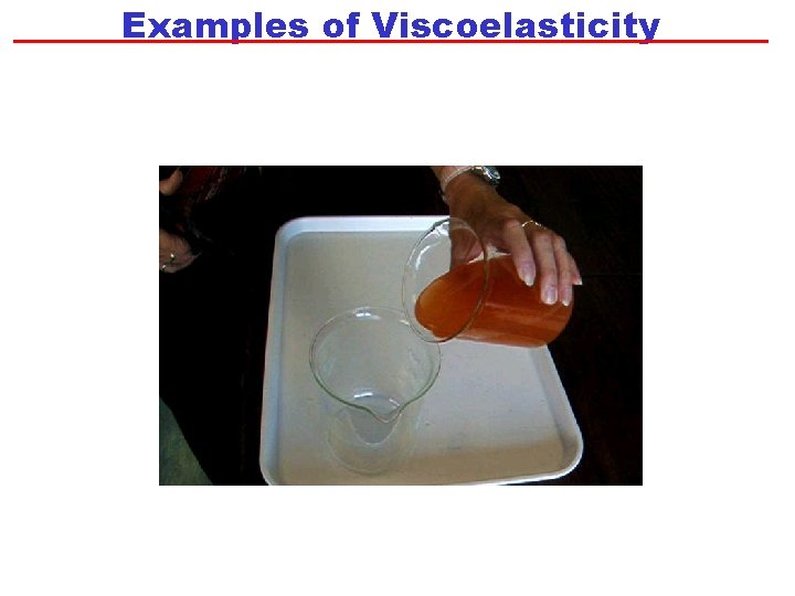
Examples of Viscoelasticity

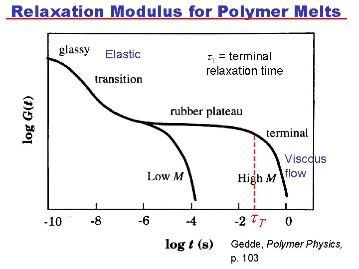
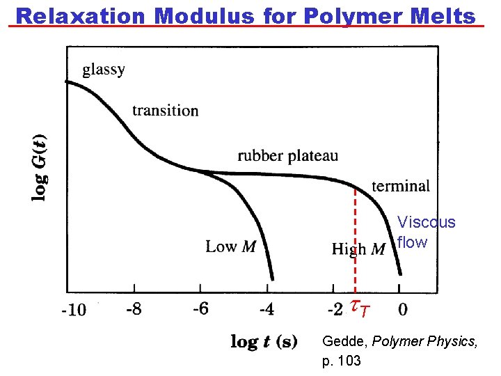
Relaxation Modulus for Polymer Melts Elastic t. T = terminal relaxation time Viscous flow t. T Gedde, Polymer Physics, p. 103

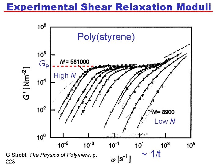
Experimental Shear Relaxation Moduli Poly(styrene) GP High N Low N G. Strobl, The Physics of Polymers, p. 223 ~ 1/t

Relaxation Modulus for Polymer Melts • At very short times, G is high. The polymer has a glassy response. • The glassy response is determined by the intramolecular bonding. • G then decreases until it reaches a “plateau modulus”, GP. The value of GP is independent of N for a given polymer: GP ~ N 0. • After a time, known as the terminal relaxation time, t. T, viscous flow starts (G decreases with time). • Experimentally, it is found that t. T is longer for polymers with a higher N. Specifically, t. T ~ N 3. 4 • Previously, we said that the relaxation time is related to ratio of h to G at the transition between elastic and viscous behaviour. Thus: t. T~h/GP

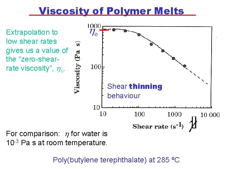
Viscosity of Polymer Melts Extrapolation to low shear rates gives us a value of the “zero-shearrate viscosity”, ho. ho Shear thinning behaviour For comparison: h for water is 10 -3 Pa s at room temperature. Poly(butylene terephthalate) at 285 ºC

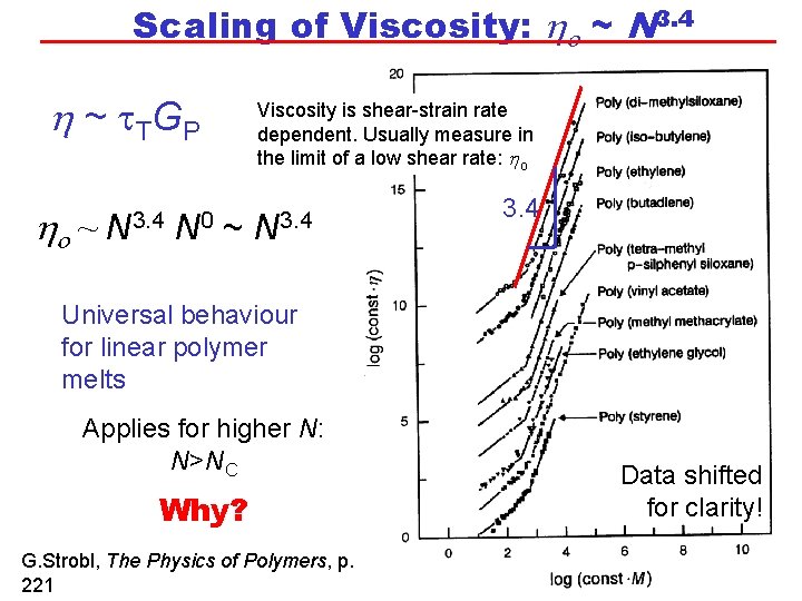
Scaling of Viscosity: ho ~ N 3. 4 h ~ t TG P ho ~ N 3. 4 N 0 Viscosity is shear-strain rate dependent. Usually measure in the limit of a low shear rate: ho ~ N 3. 4 Universal behaviour for linear polymer melts Applies for higher N: N>NC Why? G. Strobl, The Physics of Polymers, p. 221 Data shifted for clarity!

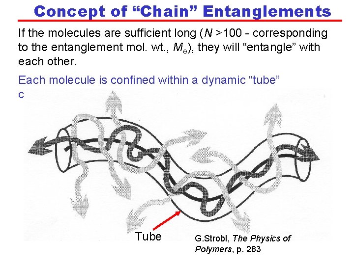
Concept of “Chain” Entanglements If the molecules are sufficient long (N >100 - corresponding to the entanglement mol. wt. , Me), they will “entangle” with each other. Each molecule is confined within a dynamic “tube” created by its neighbours. Tube G. Strobl, The Physics of Polymers, p. 283

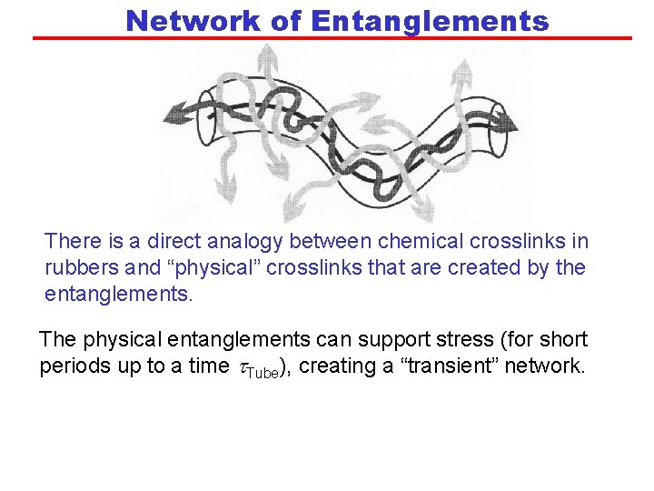
Network of Entanglements There is a direct analogy between chemical crosslinks in rubbers and “physical” crosslinks that are created by the entanglements. The physical entanglements can support stress (for short periods up to a time t. Tube), creating a “transient” network.

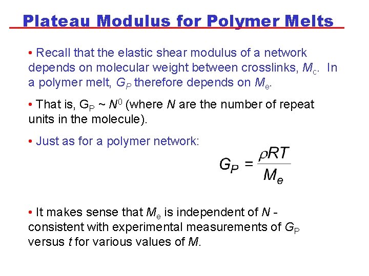
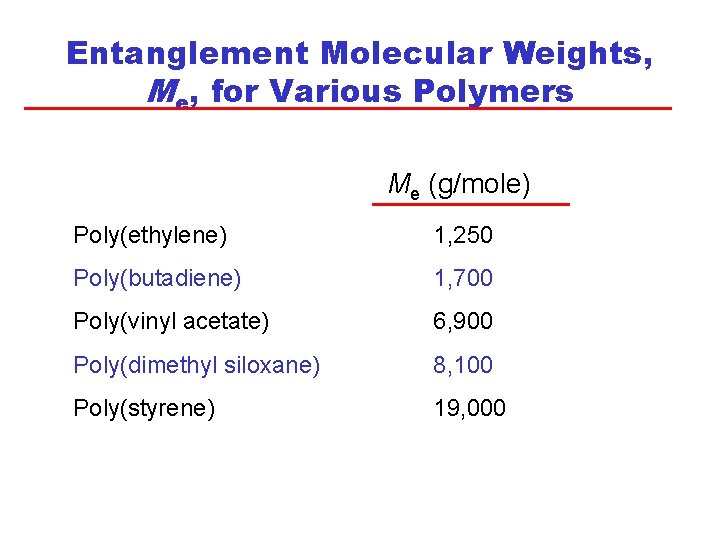
Plateau Modulus for Polymer Melts • Recall that the elastic shear modulus of a network depends on molecular weight between crosslinks, Mc. In a polymer melt, GP therefore depends on Me. • That is, GP ~ N 0 (where N are the number of repeat units in the molecule). • Just as for a polymer network: • It makes sense that Me is independent of N consistent with experimental measurements of GP versus t for various values of M.

Entanglement Molecular Weights, Me, for Various Polymers Me (g/mole) Poly(ethylene) 1, 250 Poly(butadiene) 1, 700 Poly(vinyl acetate) 6, 900 Poly(dimethyl siloxane) 8, 100 Poly(styrene) 19, 000

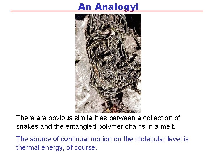
An Analogy! There are obvious similarities between a collection of snakes and the entangled polymer chains in a melt. The source of continual motion on the molecular level is thermal energy, of course.

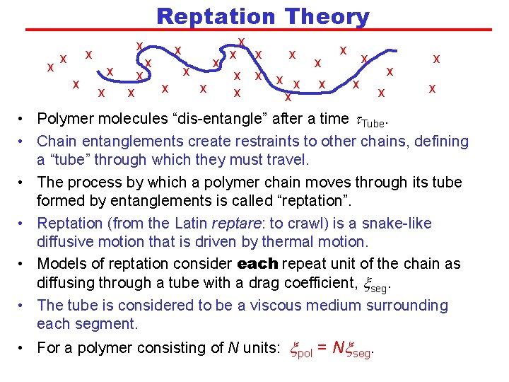
Reptation Theory x x x x x x x x x • Polymer molecules “dis-entangle” after a time t. Tube. • Chain entanglements create restraints to other chains, defining a “tube” through which they must travel. • The process by which a polymer chain moves through its tube formed by entanglements is called “reptation”. • Reptation (from the Latin reptare: to crawl) is a snake-like diffusive motion that is driven by thermal motion. • Models of reptation consider each repeat unit of the chain as diffusing through a tube with a drag coefficient, xseg. • The tube is considered to be a viscous medium surrounding each segment. • For a polymer consisting of N units: xpol = Nxseg.

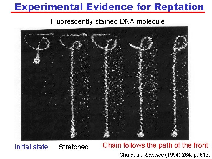
Experimental Evidence for Reptation Fluorescently-stained DNA molecule Initial state Stretched Chain follows the path of the front Chu et al. , Science (1994) 264, p. 819.

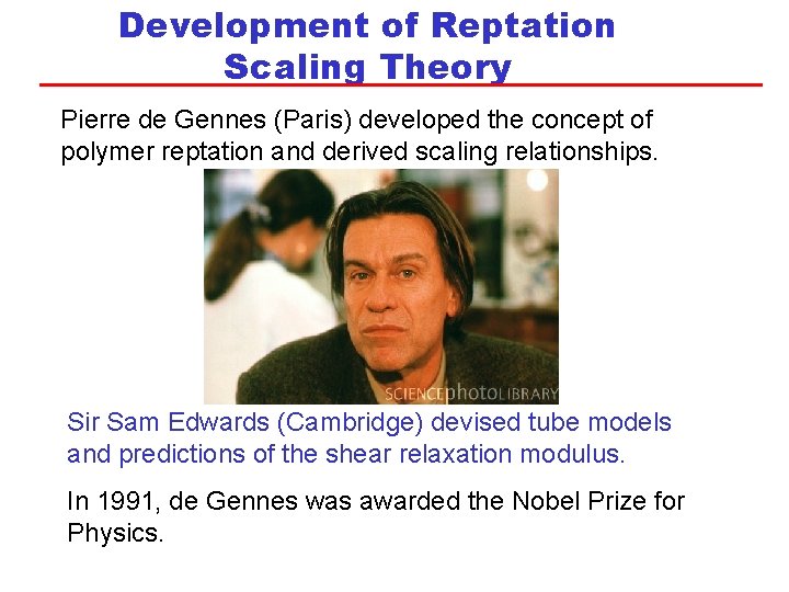
Development of Reptation Scaling Theory Pierre de Gennes (Paris) developed the concept of polymer reptation and derived scaling relationships. Sir Sam Edwards (Cambridge) devised tube models and predictions of the shear relaxation modulus. In 1991, de Gennes was awarded the Nobel Prize for Physics.

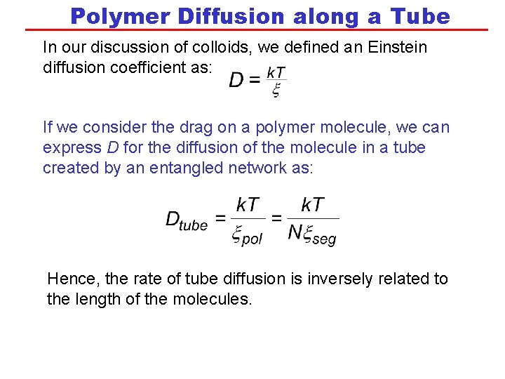
Polymer Diffusion along a Tube In our discussion of colloids, we defined an Einstein diffusion coefficient as: If we consider the drag on a polymer molecule, we can express D for the diffusion of the molecule in a tube created by an entangled network as: Hence, the rate of tube diffusion is inversely related to the length of the molecules.

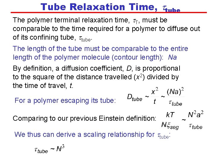
Tube Relaxation Time, ttube The polymer terminal relaxation time, t. T, must be comparable to the time required for a polymer to diffuse out of its confining tube, ttube. The length of the tube must be comparable to the entire length of the polymer molecule (contour length): Na By definition, a diffusion coefficient, D, is proportional to the square of the distance travelled (x 2) divided by the time of travel, t. For a polymer escaping its tube: Comparing to our previous Einstein definition: We thus can derive a scaling relationship for ttube:

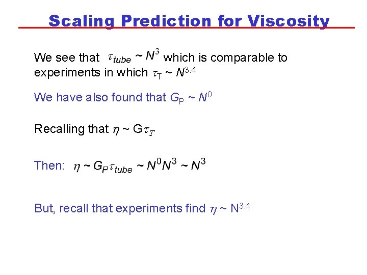
Scaling Prediction for Viscosity We see that which is comparable to experiments in which t. T ~ N 3. 4 We have also found that GP ~ N 0 Recalling that h ~ Gt. T Then: But, recall that experiments find h ~ N 3. 4

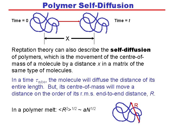
Polymer Self-Diffusion Time = 0 Time = t X Reptation theory can also describe the self-diffusion of polymers, which is the movement of the centre-ofmass of a molecule by a distance x in a matrix of the same type of molecules. In a time ttube, the molecule will diffuse the distance of its entire length. But, its centre-of-mass will move a distance on the order of its r. m. s. end-to-end distance, R. In a polymer melt: <R 2>1/2 ~ a. N 1/2 R

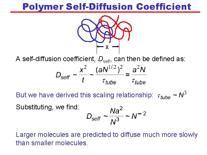
Polymer Self-Diffusion Coefficient X A self-diffusion coefficient, Dself, can then be defined as: But we have derived this scaling relationship: Substituting, we find: Larger molecules are predicted to diffuse much more slowly than smaller molecules.

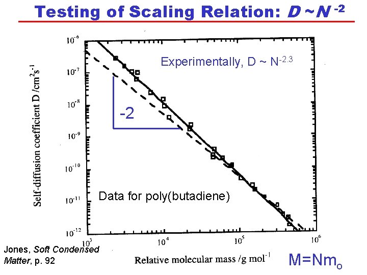
Testing of Scaling Relation: D ~N -2 Experimentally, D ~ N-2. 3 -2 Data for poly(butadiene) Jones, Soft Condensed Matter, p. 92 M=Nmo

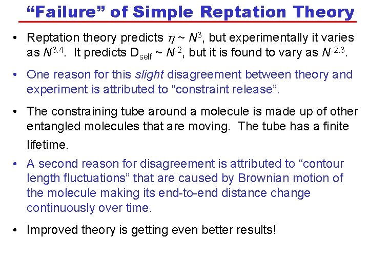
“Failure” of Simple Reptation Theory • Reptation theory predicts h ~ N 3, but experimentally it varies as N 3. 4. It predicts Dself ~ N-2, but it is found to vary as N-2. 3. • One reason for this slight disagreement between theory and experiment is attributed to “constraint release”. • The constraining tube around a molecule is made up of other entangled molecules that are moving. The tube has a finite lifetime. • A second reason for disagreement is attributed to “contour length fluctuations” that are caused by Brownian motion of the molecule making its end-to-end distance change continuously over time. • Improved theory is getting even better results!

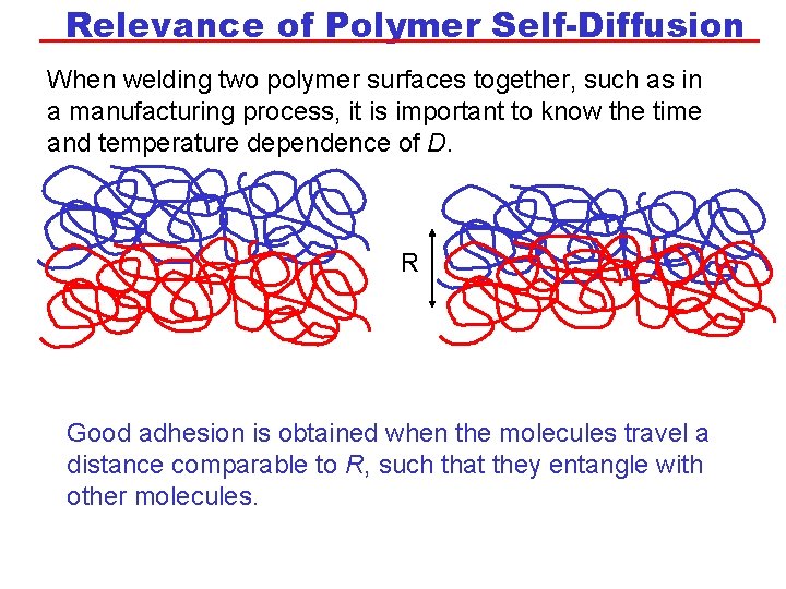
Relevance of Polymer Self-Diffusion When welding two polymer surfaces together, such as in a manufacturing process, it is important to know the time and temperature dependence of D. R Good adhesion is obtained when the molecules travel a distance comparable to R, such that they entangle with other molecules.

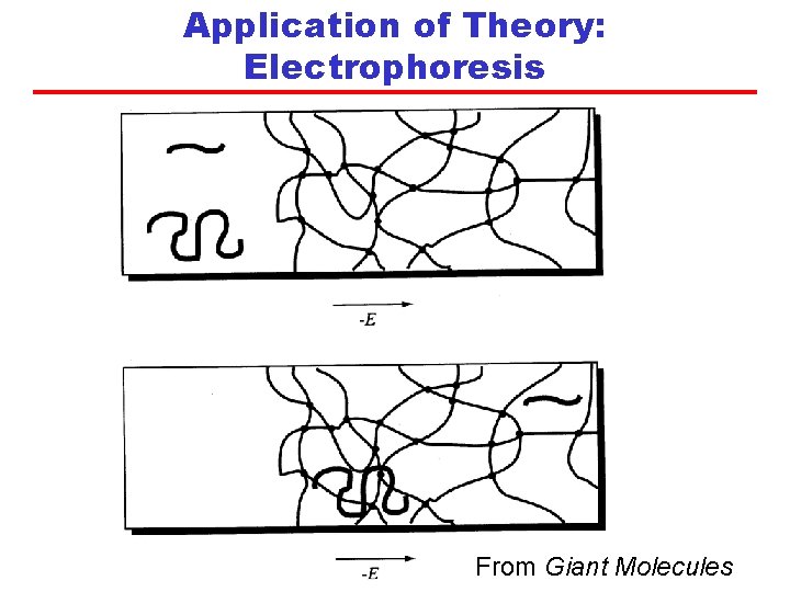
Application of Theory: Electrophoresis • DNA is a long chain molecule consisting of four different types of repeat units. • DNA can be reacted with certain enzymes to break specific bonds along its “backbone”, creating segments of various sizes. • Under an applied electric field, the segments will diffuse into a gel (crosslinked molecules in a solvent) in a process known as gel electrophoresis. • Reptation theory predicts that shorter chains will diffuse faster than longer chains. • Measuring the diffusion distances in a known time enables the determination of N for each segment and hence the position of the bonds sensitive to the enzyme.

Application of Theory: Electrophoresis From Giant Molecules

Relaxation Modulus for Polymer Melts Viscous flow t. T Gedde, Polymer Physics, p. 103

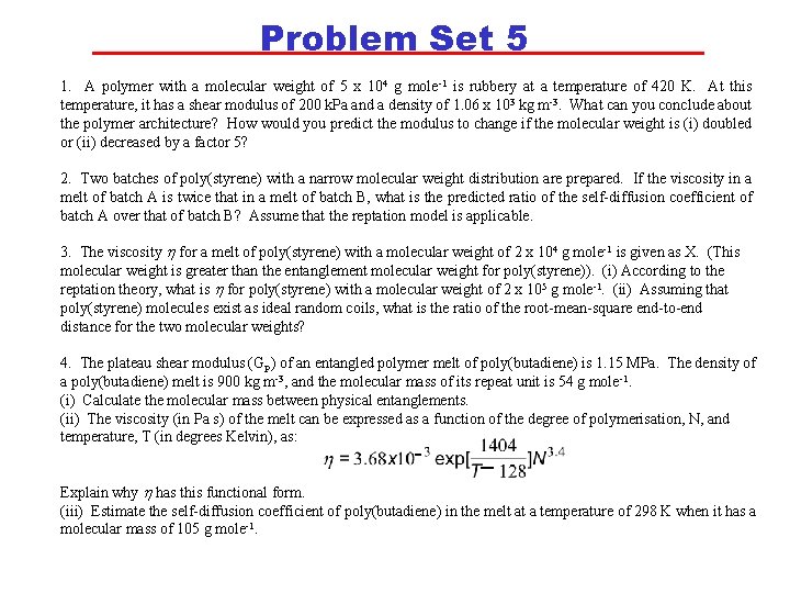
Problem Set 5 1. A polymer with a molecular weight of 5 x 104 g mole-1 is rubbery at a temperature of 420 K. At this temperature, it has a shear modulus of 200 k. Pa and a density of 1. 06 x 103 kg m-3. What can you conclude about the polymer architecture? How would you predict the modulus to change if the molecular weight is (i) doubled or (ii) decreased by a factor 5? 2. Two batches of poly(styrene) with a narrow molecular weight distribution are prepared. If the viscosity in a melt of batch A is twice that in a melt of batch B, what is the predicted ratio of the self-diffusion coefficient of batch A over that of batch B? Assume that the reptation model is applicable. 3. The viscosity h for a melt of poly(styrene) with a molecular weight of 2 x 104 g mole-1 is given as X. (This molecular weight is greater than the entanglement molecular weight for poly(styrene)). (i) According to the reptation theory, what is h for poly(styrene) with a molecular weight of 2 x 105 g mole-1. (ii) Assuming that poly(styrene) molecules exist as ideal random coils, what is the ratio of the root-mean-square end-to-end distance for the two molecular weights? 4. The plateau shear modulus (GP) of an entangled polymer melt of poly(butadiene) is 1. 15 MPa. The density of a poly(butadiene) melt is 900 kg m-3, and the molecular mass of its repeat unit is 54 g mole-1. (i) Calculate the molecular mass between physical entanglements. (ii) The viscosity (in Pa s) of the melt can be expressed as a function of the degree of polymerisation, N, and temperature, T (in degrees Kelvin), as: Explain why h has this functional form. (iii) Estimate the self-diffusion coefficient of poly(butadiene) in the melt at a temperature of 298 K when it has a molecular mass of 105 g mole-1.