Last lecture summary Testdata and Cross Validation testing

Last lecture summary

Test-data and Cross Validation

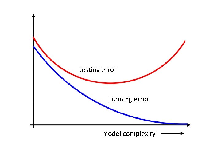
testing error training error model complexity

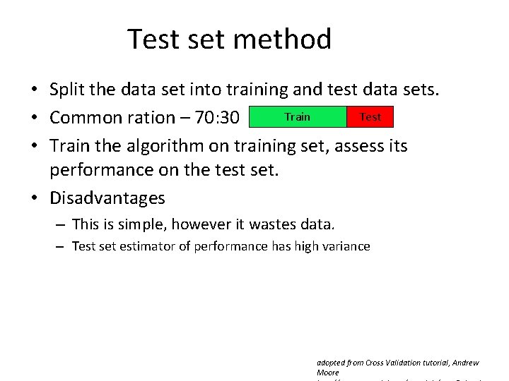
Test set method • Split the data set into training and test data sets. Train Test • Common ration – 70: 30 • Train the algorithm on training set, assess its performance on the test set. • Disadvantages – This is simple, however it wastes data. – Test set estimator of performance has high variance adopted from Cross Validation tutorial, Andrew Moore

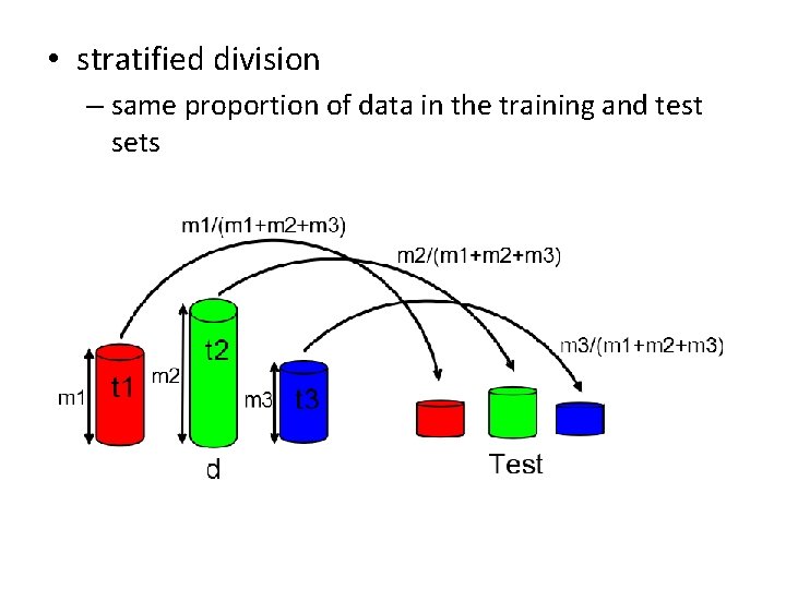
• stratified division – same proportion of data in the training and test sets

• Training error can not be used as an indicator of model’s performance due to overfitting. • Training data set - train a range of models, or a given model with a range of values for its parameters. • Compare them on independent data – Validation set. – If the model design is iterated many times, then some overfitting to the validation data can occur and so it may be necessary to keep aside a third • Test set on which the performance of the selected model is finally evaluated.

LOOCV 1. choose one data point 2. remove it from the set 3. fit the remaining data points 4. note your error using the removed data point as test Repeat these steps for all points. When you are done report the mean square error (in case of regression).

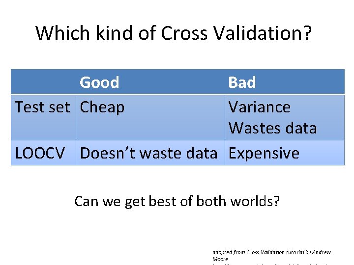
Which kind of Cross Validation? Good Test set Cheap Bad Variance Wastes data LOOCV Doesn’t waste data Expensive Can we get best of both worlds? adopted from Cross Validation tutorial by Andrew Moore

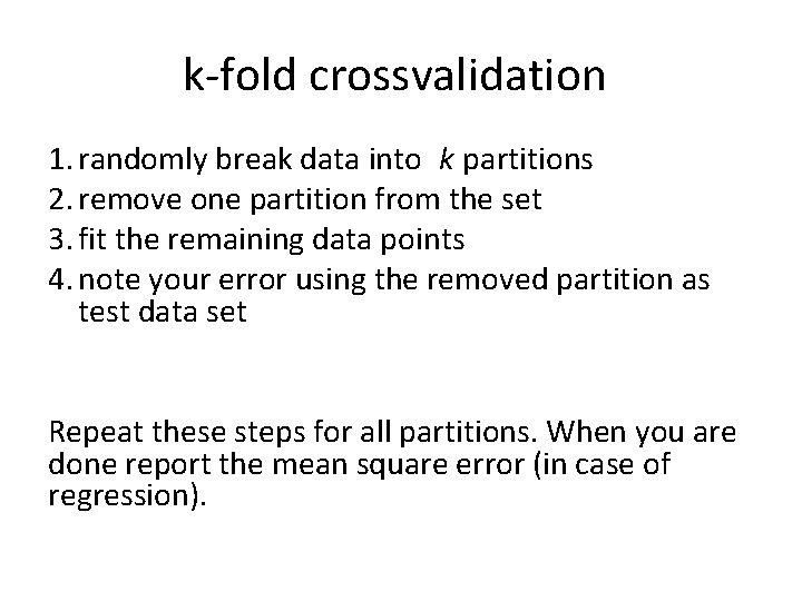
k-fold crossvalidation 1. randomly break data into k partitions 2. remove one partition from the set 3. fit the remaining data points 4. note your error using the removed partition as test data set Repeat these steps for all partitions. When you are done report the mean square error (in case of regression).

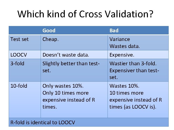
Which kind of Cross Validation? Test set Good Cheap. Bad Variance Wastes data. LOOCV Doesn’t waste data. Expensive. 3 -fold Slightly better than testset. 10 -fold Only wastes 10%. Only 10 times more expensive instead of R times. Wastier than 3 -fold. Expensiver than testset. Wastes 10%. 10 times more expensive instead of R times (as LOOCV is). R-fold is identical to LOOCV

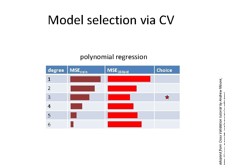
Model selection via CV polynomial regression 1 2 3 4 5 6 MSEtrain MSE 10 -fold Choice adopted from Cross Validation tutorial by Andrew Moore, degree

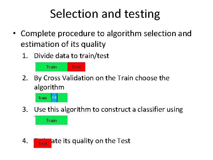
Selection and testing • Complete procedure to algorithm selection and estimation of its quality 1. Divide data to train/test Train Test 2. By Cross Validation on the Train choose the algorithm Train Val 3. Use this algorithm to construct a classifier using Train 4. Estimate its quality on the Test

Nearest Neighbors Classification

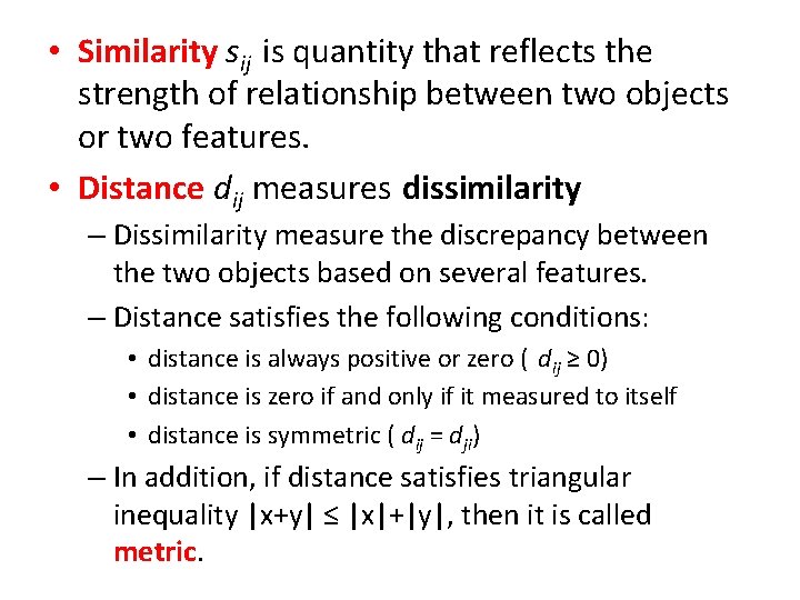
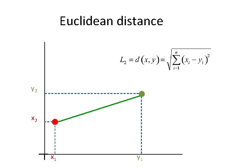
• Similarity sij is quantity that reflects the strength of relationship between two objects or two features. • Distance dij measures dissimilarity – Dissimilarity measure the discrepancy between the two objects based on several features. – Distance satisfies the following conditions: • distance is always positive or zero ( dij ≥ 0) • distance is zero if and only if it measured to itself • distance is symmetric ( dij = dji) – In addition, if distance satisfies triangular inequality |x+y| ≤ |x|+|y|, then it is called metric.

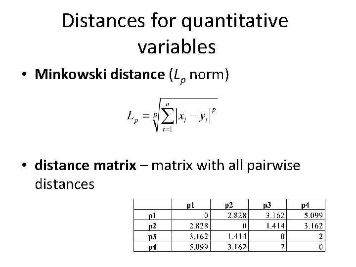
Distances for quantitative variables • Minkowski distance (Lp norm) • distance matrix – matrix with all pairwise distances

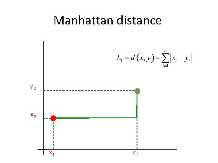
Manhattan distance y 2 x 1 y 1

Euclidean distance y 2 x 1 y 1

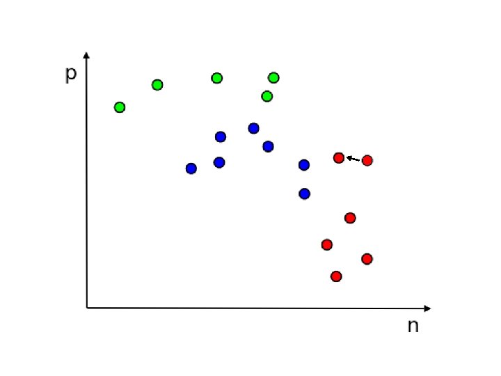
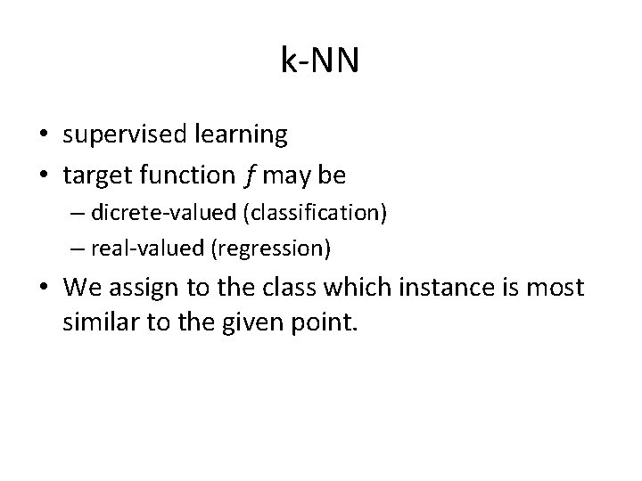
k-NN • supervised learning • target function f may be – dicrete-valued (classification) – real-valued (regression) • We assign to the class which instance is most similar to the given point.

• k-NN is a lazy learner • lazy learning – generalization beyond the training data is delayed until a query is made to the system – opposed to eager learning – system tries to generalize the training data before receiving queries

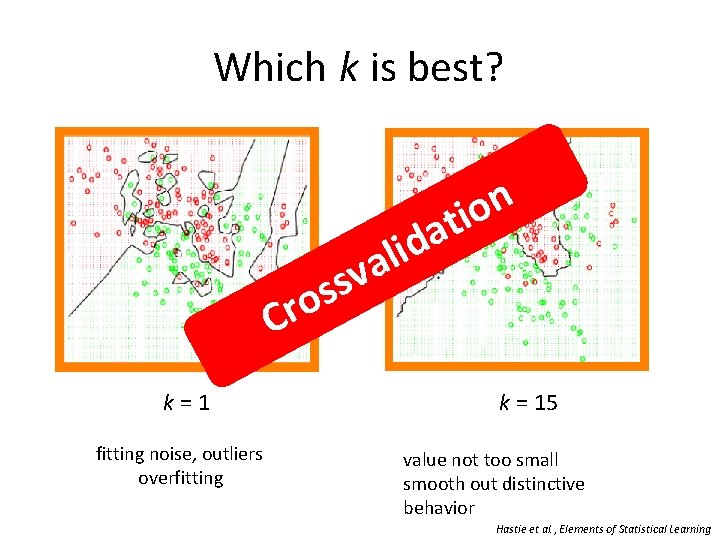
Which k is best? v s os Cr k = 1 fitting noise, outliers overfitting n o ti a d i l a k = 15 value not too small smooth out distinctive behavior Hastie et al. , Elements of Statistical Learning

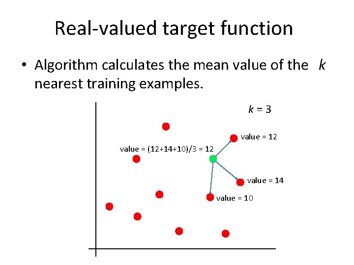
Real-valued target function • Algorithm calculates the mean value of the k nearest training examples. k = 3 value = 12 value = (12+14+10)/3 = 12 value = 14 value = 10

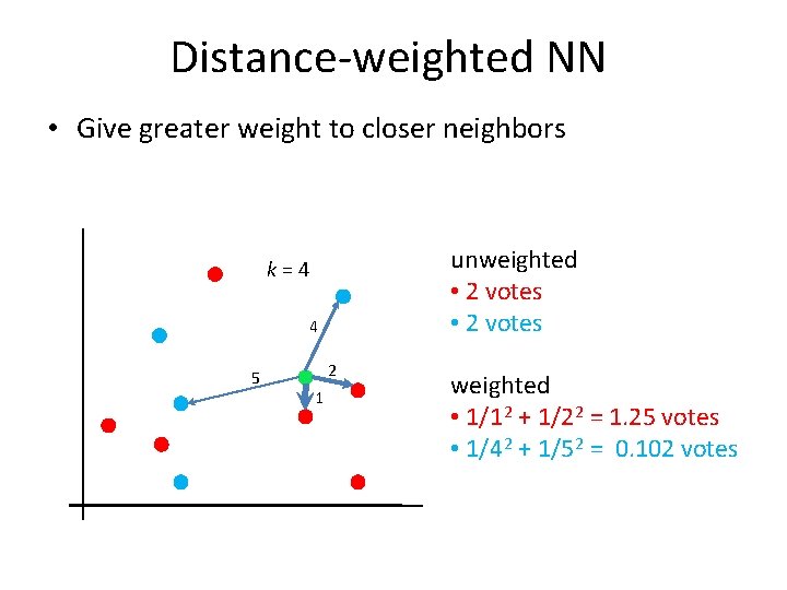
Distance-weighted NN • Give greater weight to closer neighbors unweighted • 2 votes k = 4 4 5 2 1 weighted • 1/1 2 + 1/2 2 = 1. 25 votes • 1/4 2 + 1/5 2 = 0. 102 votes

k-NN issues • Curse of dimensionality is a problem. • Significant computation may be required to process each new query. • To find nearest neighbors one has to evaluate full distance matrix. • Efficient indexing of stored training examples helps – kd-tree

Cluster Analysis (i. e. new stuff)

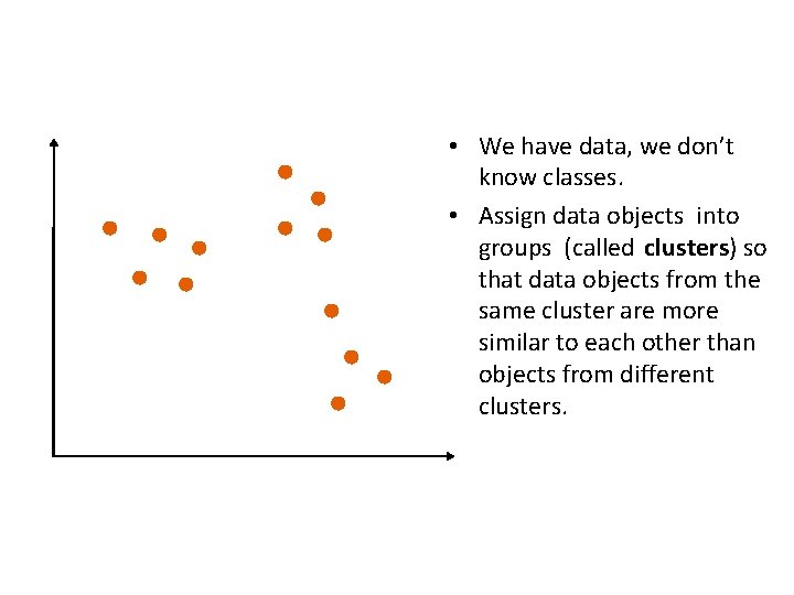
• We have data, we don’t know classes. • Assign data objects into groups (called clusters) so that data objects from the same cluster are more similar to each other than objects from different clusters.

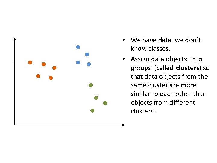
• We have data, we don’t know classes. • Assign data objects into groups (called clusters) so that data objects from the same cluster are more similar to each other than objects from different clusters.

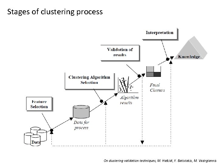
Stages of clustering process On clustering validation techniques, M. Halkidi, Y. Batistakis, M. Vazirgiannis

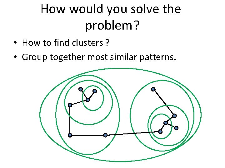
How would you solve the problem? • How to find clusters ? • Group together most similar patterns.

Single linkage based on A Tutorial on Clustering Algorithms http: //home. dei. polimi. it/matteucc/Clustering/tutorial_html/hierarchical. ht

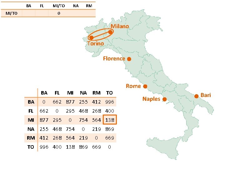
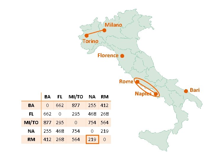
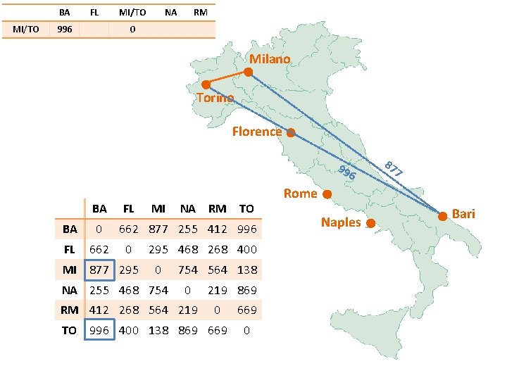
BA FL MI/TO NA RM 0 Milano Torino Florence BA FL BA 0 FL 662 MI 877 295 MI NA RM TO 662 877 255 412 996 0 295 468 268 400 0 NA 255 468 754 564 138 0 RM 412 268 564 219 869 0 TO 996 400 138 869 669 0 Rome Naples Bari

BA MI/TO FL 877 MI/TO NA RM 0 Milano Torino Florence 99 6 BA FL BA 0 FL 662 MI 877 295 MI NA RM TO 662 877 255 412 996 0 295 468 268 400 0 NA 255 468 754 564 138 0 RM 412 268 564 219 869 0 TO 996 400 138 869 669 0 87 7 Rome Naples Bari

MI/TO BA FL MI/TO 877 295 0 NA RM Milano 40 0 5 29 Torino Florence BA FL BA 0 FL 662 MI 877 295 MI NA RM TO 662 877 255 412 996 0 295 468 268 400 0 NA 255 468 754 564 138 0 RM 412 268 564 219 869 0 TO 996 400 138 869 669 0 Rome Naples Bari

MI/TO BA FL MI/TO NA RM 877 295 0 754 Milano Torino 86 9 BA FL BA 0 FL 662 MI 877 295 MI NA RM TO 662 877 255 412 996 0 295 468 268 400 0 NA 255 468 754 564 138 0 RM 412 268 564 219 869 0 TO 996 400 138 869 669 0 4 75 Florence Rome Naples Bari

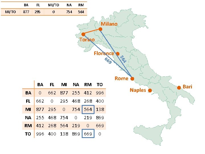
MI/TO BA FL MI/TO NA RM 877 295 0 754 564 Milano Torino Florence 9 BA FL BA 0 FL 662 MI 877 295 MI NA RM TO 662 877 255 412 996 0 295 468 268 400 0 NA 255 468 754 564 138 0 RM 412 268 564 219 869 0 TO 996 400 138 869 669 0 4 56 66 Rome Naples Bari

Milano Torino Florence Rome BA FL MI/TO NA RM BA 0 662 877 255 412 FL 662 0 295 468 268 0 754 564 MI/TO 877 295 NA 255 468 754 0 219 RM 412 268 564 219 0 Naples Bari

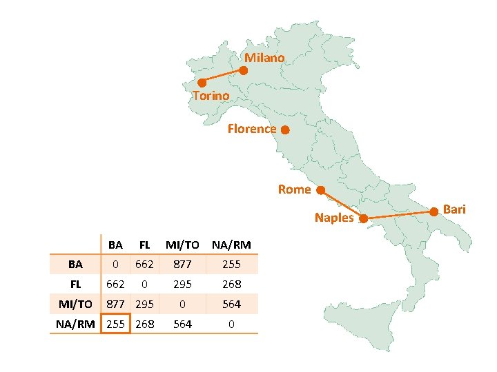
Milano Torino Florence Rome Naples BA FL MI/TO NA/RM BA 0 662 877 255 FL 662 0 295 268 0 564 0 MI/TO 877 295 NA/RM 255 268 Bari

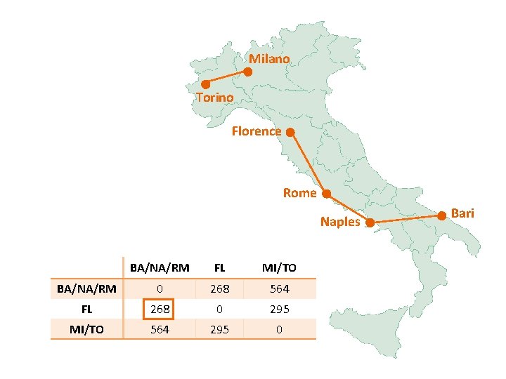
Milano Torino Florence Rome Naples BA/NA/RM FL MI/TO BA/NA/RM 0 268 564 FL 268 0 295 MI/TO 564 295 0 Bari

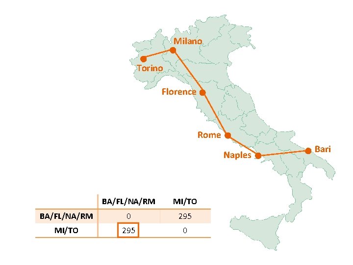
Milano Torino Florence Rome Naples BA/FL/NA/RM MI/TO BA/FL/NA/RM 0 295 MI/TO 295 0 Bari

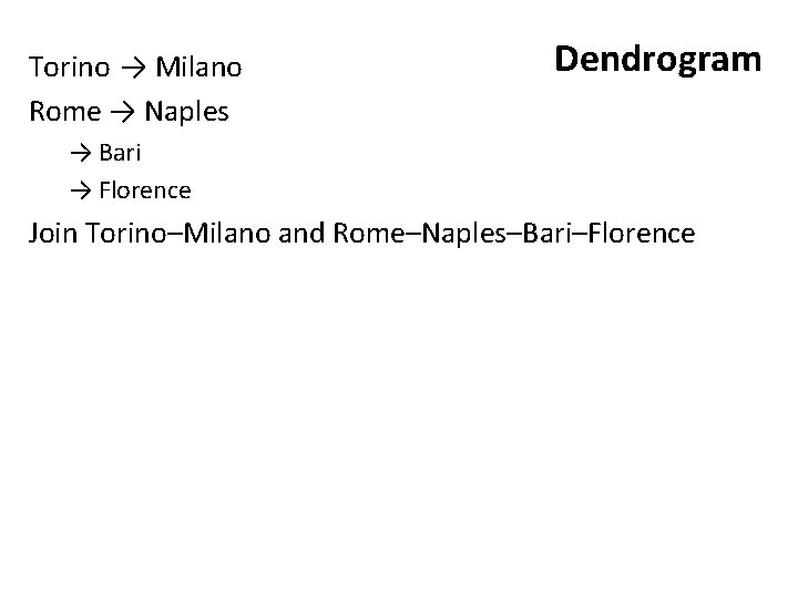
Torino → Milano Rome → Naples Dendrogram → Bari → Florence Join Torino–Milano and Rome–Naples–Bari–Florence

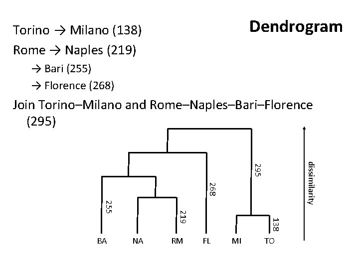
Dendrogram Torino → Milano (138) Rome → Naples (219) → Bari (255) → Florence (268) Join Torino–Milano and Rome–Naples–Bari–Florence (295) dissimilarity 295 268 NA RM 138 219 255 BA FL MI TO

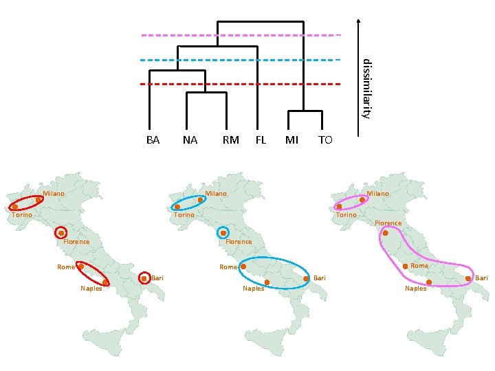
dissimilarity BA NA Milano RM FL MI TO Milano Torino Florence Rome Bari Naples Florence Bari Naples

Complete linkage

BA FL MI/TO NA RM 0 Milano Torino Florence BA FL BA 0 FL 662 MI 877 295 MI NA RM TO 662 877 255 412 996 0 295 468 268 400 0 NA 255 468 754 564 138 0 RM 412 268 564 219 869 0 TO 996 400 138 869 669 0 Rome Naples Bari

BA MI/TO FL 996 MI/TO NA RM 0 Milano Torino Florence 99 6 BA FL BA 0 FL 662 MI 877 295 MI NA RM TO 662 877 255 412 996 0 295 468 268 400 0 NA 255 468 754 564 138 0 RM 412 268 564 219 869 0 TO 996 400 138 869 669 0 87 7 Rome Naples Bari

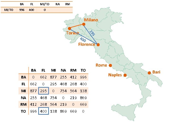
MI/TO BA FL MI/TO 996 400 0 NA RM Milano 40 0 5 29 Torino Florence BA FL BA 0 FL 662 MI 877 295 MI NA RM TO 662 877 255 412 996 0 295 468 268 400 0 NA 255 468 754 564 138 0 RM 412 268 564 219 869 0 TO 996 400 138 869 669 0 Rome Naples Bari

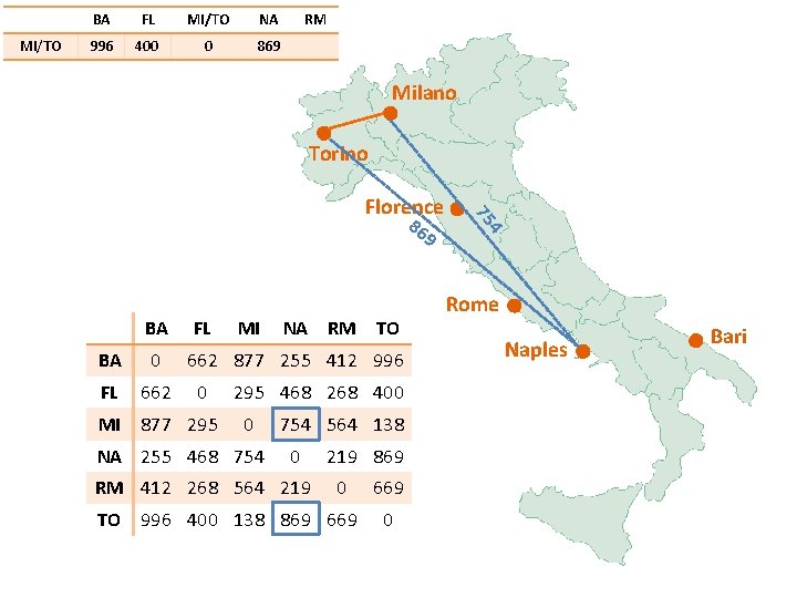
MI/TO BA FL MI/TO NA RM 996 400 0 869 Milano Torino 86 9 BA FL BA 0 FL 662 MI 877 295 MI NA RM TO 662 877 255 412 996 0 295 468 268 400 0 NA 255 468 754 564 138 0 RM 412 268 564 219 869 0 TO 996 400 138 869 669 0 4 75 Florence Rome Naples Bari

MI/TO BA FL MI/TO NA RM 996 400 0 869 669 Milano Torino Florence 9 BA FL BA 0 FL 662 MI 877 295 MI NA RM TO 662 877 255 412 996 0 295 468 268 400 0 NA 255 468 754 564 138 0 RM 412 268 564 219 869 0 TO 996 400 138 869 669 0 4 56 66 Rome Naples Bari

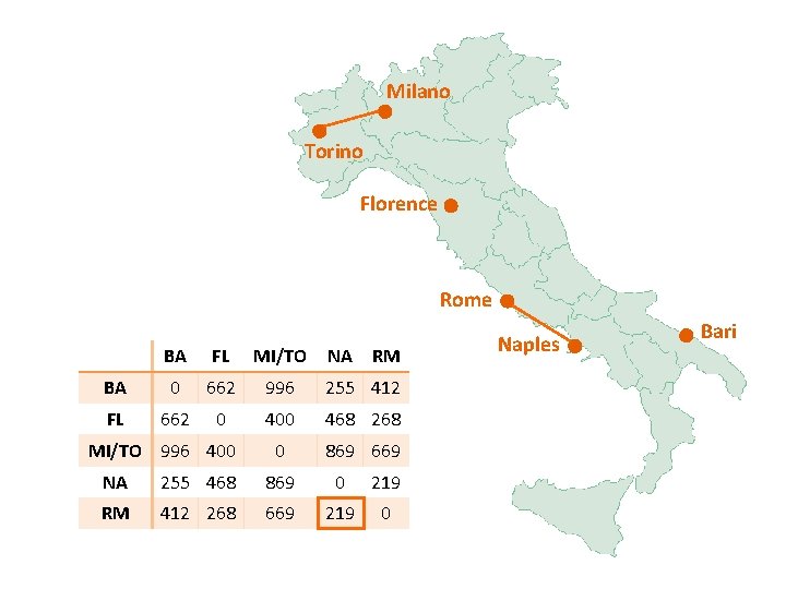
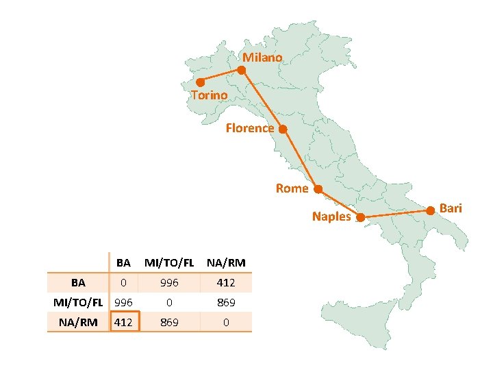
Milano Torino Florence Rome BA FL MI/TO NA RM BA 0 662 996 255 412 FL 662 0 400 468 268 0 869 669 MI/TO 996 400 NA 255 468 869 0 219 RM 412 268 669 219 0 Naples Bari

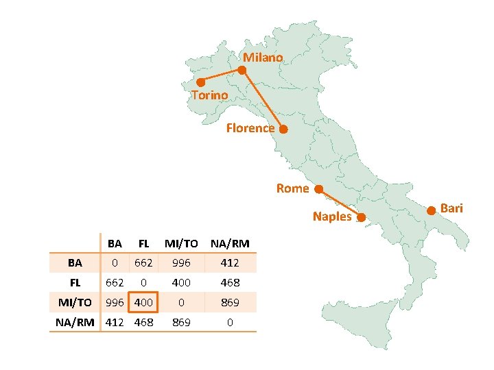
Milano Torino Florence Rome Naples BA FL MI/TO NA/RM BA 0 662 996 412 FL 662 0 400 468 0 869 0 MI/TO 996 400 NA/RM 412 468 Bari

Milano Torino Florence Rome Naples BA BA MI/TO/FL NA/RM 0 996 412 0 869 0 MI/TO/FL 996 NA/RM 412 Bari

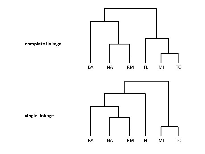
complete linkage BA NA RM FL MI TO single linkage

Average linkage

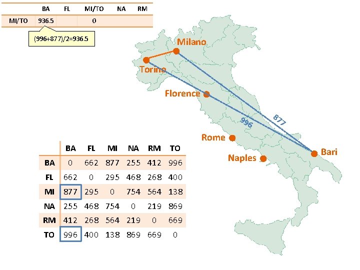
BA MI/TO FL MI/TO 936. 5 NA RM 0 (996+877)/2=936. 5 Milano Torino Florence 99 6 BA FL BA 0 FL 662 MI 877 295 MI NA RM TO 662 877 255 412 996 0 295 468 268 400 0 NA 255 468 754 564 138 0 RM 412 268 564 219 869 0 TO 996 400 138 869 669 0 87 7 Rome Naples Bari

Centroid linkage

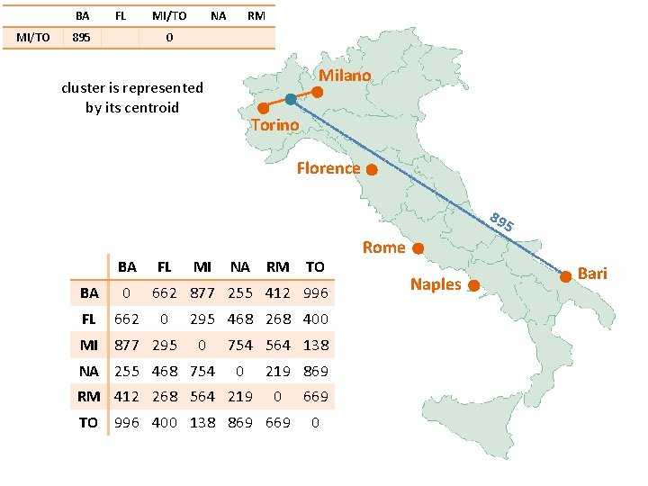
BA MI/TO FL 895 MI/TO NA RM 0 Milano cluster is represented by its centroid Torino Florence 89 5 BA FL BA 0 FL 662 MI 877 295 MI NA RM TO 662 877 255 412 996 0 295 468 268 400 0 NA 255 468 754 564 138 0 RM 412 268 564 219 869 0 TO 996 400 138 869 669 0 Rome Naples Bari

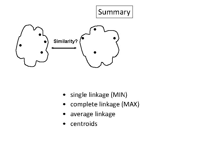
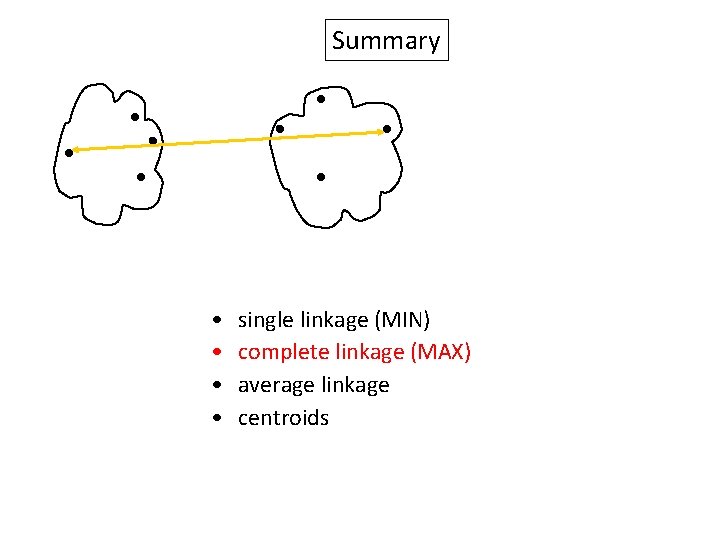
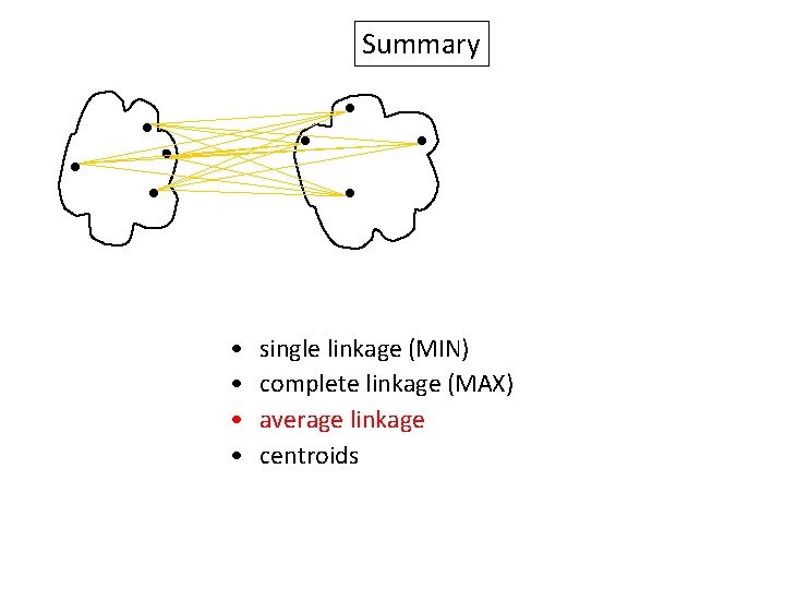
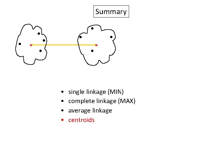
Summary Similarity? • • single linkage (MIN) complete linkage (MAX) average linkage centroids

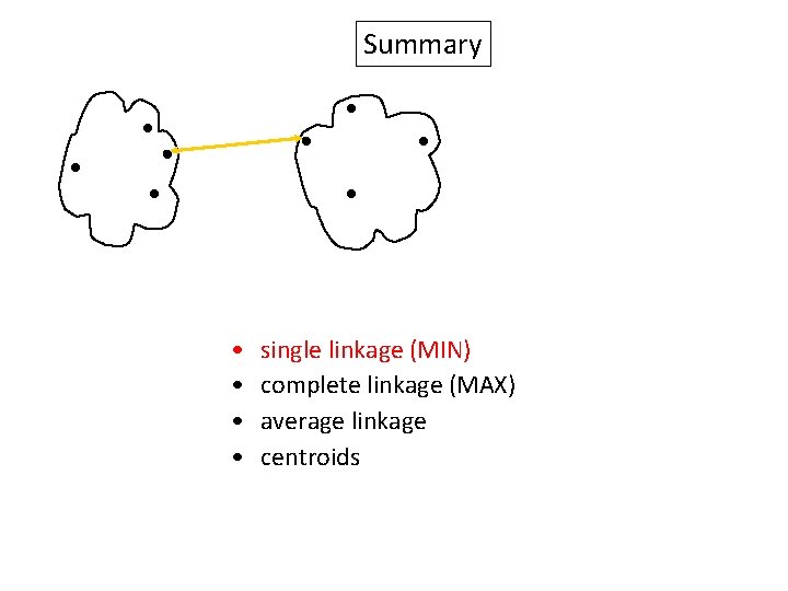
Summary • • single linkage (MIN) complete linkage (MAX) average linkage centroids

Summary • • single linkage (MIN) complete linkage (MAX) average linkage centroids

Summary • • single linkage (MIN) complete linkage (MAX) average linkage centroids

Summary • • single linkage (MIN) complete linkage (MAX) average linkage centroids

Ward’s linkage (method)

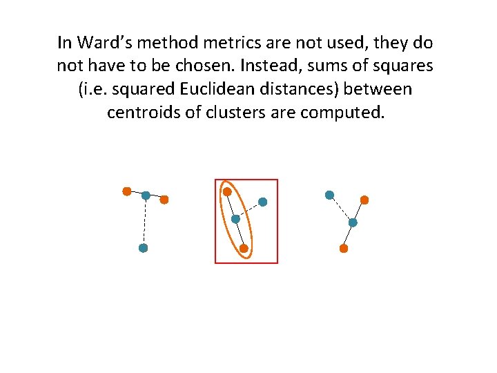
In Ward’s method metrics are not used, they do not have to be chosen. Instead, sums of squares (i. e. squared Euclidean distances) between centroids of clusters are computed.

• Ward's method says that the distance between two clusters, A and B, is how much the sum of squares will increase when we merge them. • At the beginning of clustering, the sum of squares starts out at zero (because every point is in its own cluster) and then grows as we merge clusters. • Ward‘s method keeps this growth as small as possible.

Types of clustering • hierarchical – groups data with a sequence of nested partitions • agglomerative – bottom-up – Start with each data point as one cluster, join the clusters up to the situation when all points form one cluster. • divisive – top-down – Initially all objects are in one cluster, then the cluster is subdivided into smaller and smaller pieces. • partitional – divides data points into some prespecified number of clusters without the hierarchical structure – i. e. divides the space

Hierarchical clustering • Agglomerative methods are used more widely. • Divisive methods need to consider (2 N − 1) possible subset divisions, which is very computationally intensive. – computational difficulties of finding the optimum partitions • Divisive clustering methods are better at finding large clusters than hierarchical methods.

Hierarchical clustering • Disadvantages – High computational complexity – at least O(N 2). • Needs to calculate all mutual distances. – Inability to adjust once the splitting or merging is performed • no undo

k-means • How to avoid the computing of all mutual distances? • Calculate distances from representatives (centroids) of clusters. • Advantage: number of centroids is much lower than the number of data points. • Disadvantage: number of centroids k must be given in advance

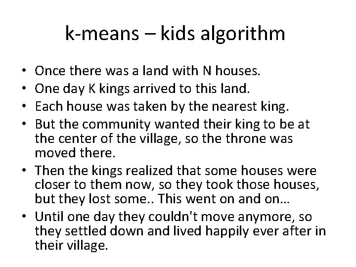
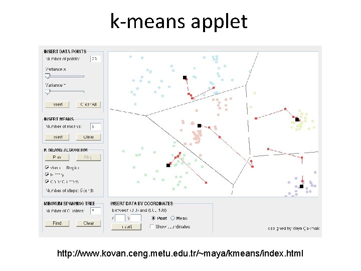
k-means – kids algorithm Once there was a land with N houses. One day K kings arrived to this land. Each house was taken by the nearest king. But the community wanted their king to be at the center of the village, so the throne was moved there. • Then the kings realized that some houses were closer to them now, so they took those houses, but they lost some. . This went on and on… • Until one day they couldn't move anymore, so they settled down and lived happily ever after in their village. • •

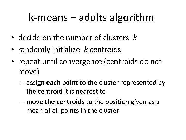
k-means – adults algorithm • decide on the number of clusters k • randomly initialize k centroids • repeat until convergence (centroids do not move) – assign each point to the cluster represented by the centroid it is nearest to – move the centroids to the position given as a mean of all points in the cluster

k-means applet http: //www. kovan. ceng. metu. edu. tr/~maya/kmeans/index. html

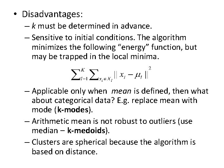
• Disadvantages: – k must be determined in advance. – Sensitive to initial conditions. The algorithm minimizes the following “energy” function, but may be trapped in the local minima. – Applicable only when mean is defined, then what about categorical data? E. g. replace mean with mode (k-modes). – Arithmetic mean is not robust to outliers (use median – k-medoids). – Clusters are spherical because the algorithm is based on distance.

Cluster validation • How many clusters are there in data set? • Does the resulting clustering scheme fit our data set? • Is there a better partitioning for the data set? • The quantitative evaluations of the clustering results are known under the general term cluster validity methods.

• external – evaluate clustering results based on the knowledge of the correct class labels • internal – no correct class labels are available, the quality estimate is based on the information intrinsic to the data alone • relative – several different classifications of one set of data are compared using the same algorithm of classification with different parameters

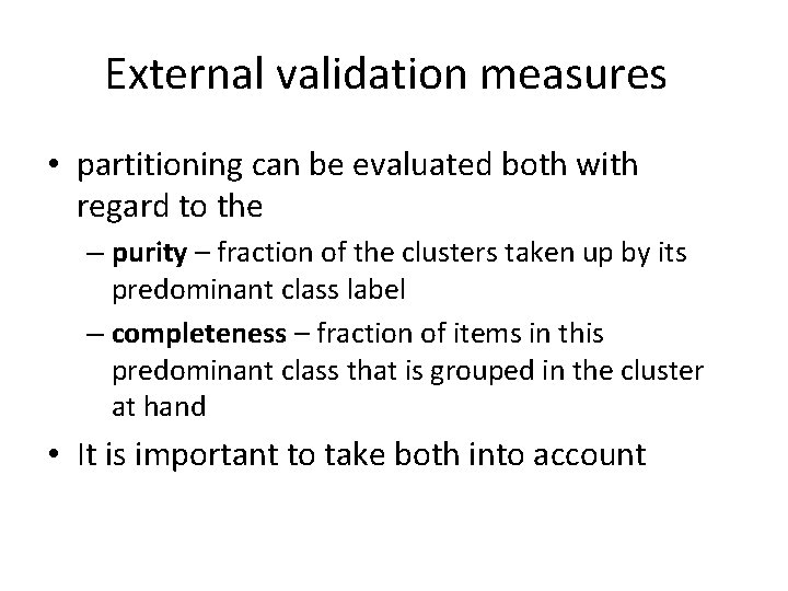
External validation measures • partitioning can be evaluated both with regard to the – purity – fraction of the clusters taken up by its predominant class label – completeness – fraction of items in this predominant class that is grouped in the cluster at hand • It is important to take both into account

• binary measures – based on the contingency table of the pairwise assignment of data items – we have two divisions of data consisting of N objects (S = {S 1 … SN}): • original data set (i. e. known) C = {C 1, …, Cn} • generated (i. e. after clustering) P = {P 1, …, Pm}

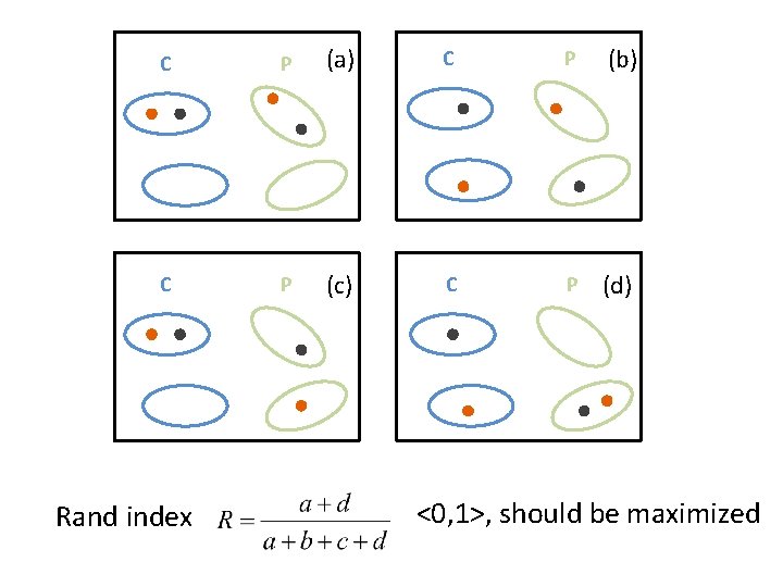
C P (a) C P (b) C P (c) C P (d) Rand index <0, 1>, should be maximized

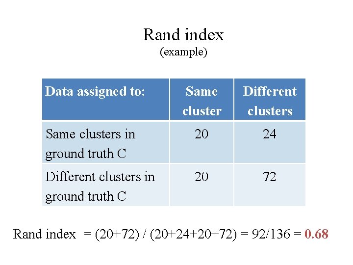
Rand index (example) Data assigned to: Same cluster Different clusters Same clusters in ground truth C 20 24 Different clusters in ground truth C 20 72 Rand index = (20+72) / (20+24+20+72) = 92/136 = 0. 68

Cophenetic correlation coefficient • How good is the hierarchical clustering that we just performed? • Meaning how faithfully a dendrogram preserves the pairwise distances between the original data points? • To calculate it we need two matrices: distance matrix and cophenetic matrix.

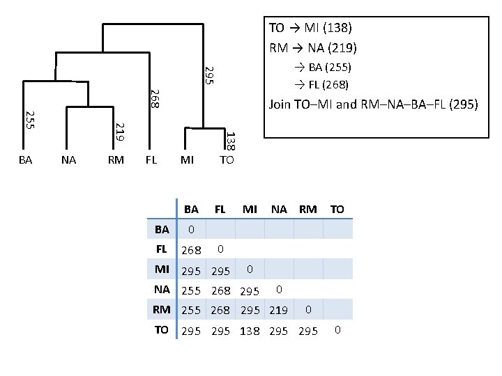
TO → MI (138) RM → NA (219) 295 → BA (255) → FL (268) 268 NA RM 138 219 255 BA Join TO–MI and RM–NA–BA–FL (295) FL MI BA BA 0 FL 268 TO FL MI NA RM TO 0 MI 295 0 NA 255 268 295 0 RM 255 268 295 219 0 TO 295 138 295 0

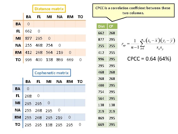
Distance matrix BA FL BA 0 FL 662 MI 877 295 MI NA RM TO 0 0 NA 255 468 754 0 RM 412 268 564 219 0 TO 996 400 138 869 669 0 Cophenetic matrix BA BA 0 FL 268 FL MI NA RM TO 0 MI 295 0 NA 255 268 295 0 RM 255 268 295 219 0 TO 295 138 295 0 CPCC is a correlation coeffcient between these two columns. Dist CP 662 268 877 295 255 412 255 996 295 295 468 268 268 400 295 754 295 564 295 138 219 869 295 669 295 CPCC = 0. 64 (64%)

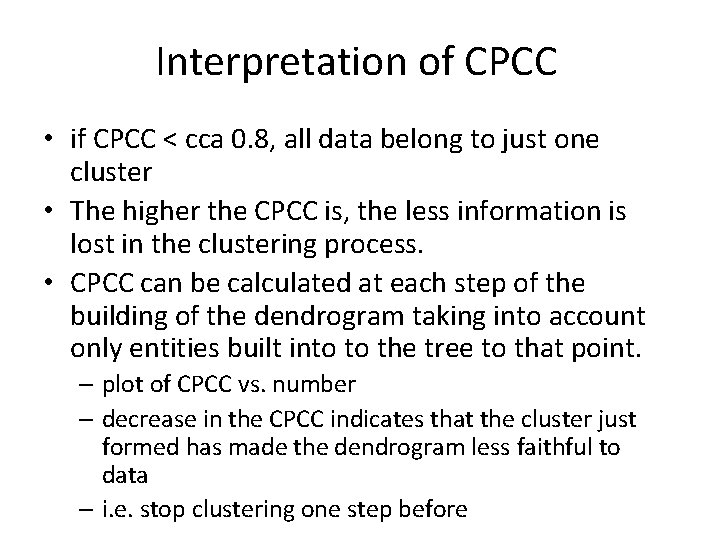
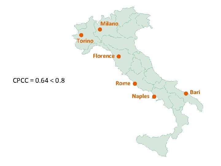
Interpretation of CPCC • if CPCC < cca 0. 8, all data belong to just one cluster • The higher the CPCC is, the less information is lost in the clustering process. • CPCC can be calculated at each step of the building of the dendrogram taking into account only entities built into to the tree to that point. – plot of CPCC vs. number – decrease in the CPCC indicates that the cluster just formed has made the dendrogram less faithful to data – i. e. stop clustering one step before

Milano Torino Florence CPCC = 0. 64 < 0. 8 Rome Naples Bari

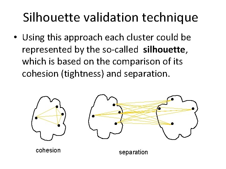
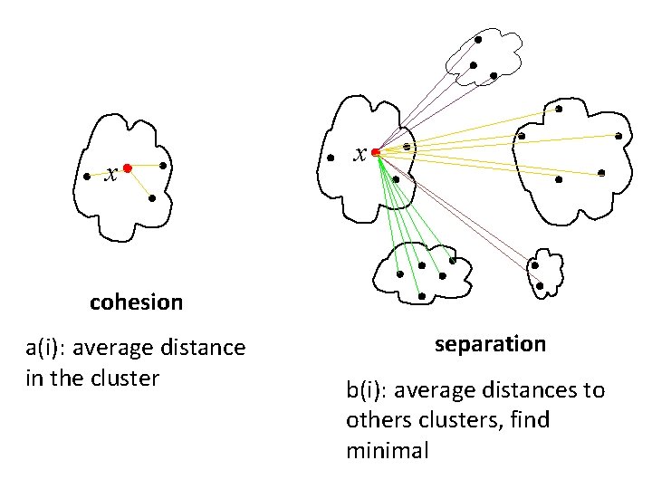
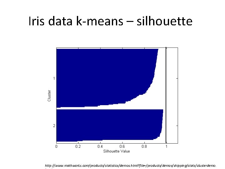
Silhouette validation technique • Using this approach each cluster could be represented by the so-called silhouette, which is based on the comparison of its cohesion (tightness) and separation. cohesion separation

• In this technique, several measures can be calculated: 1. silhouette width for each sample • you’ll see later why I call these numbers “width” 2. average silhouette width for each cluster 3. overall average silhouette width for a total data set

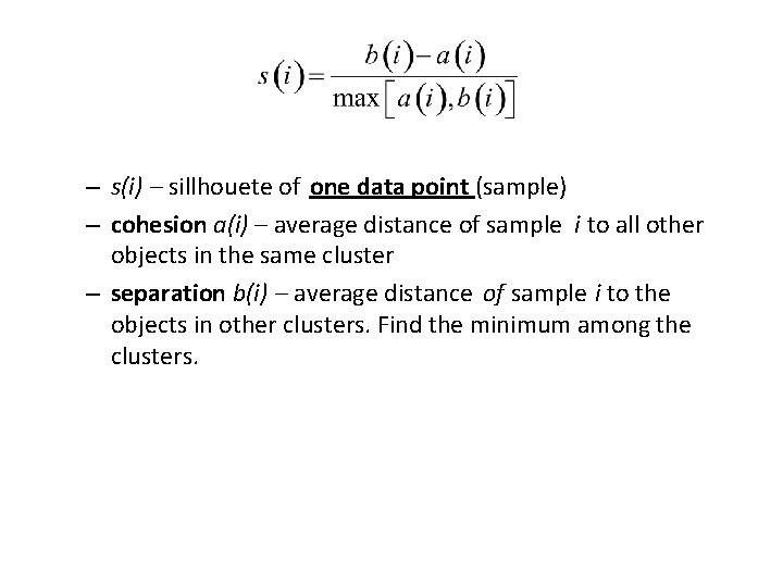
– s(i) – sillhouete of one data point (sample) – cohesion a(i) – average distance of sample i to all other objects in the same cluster – separation b(i) – average distance of sample i to the objects in other clusters. Find the minimum among the clusters.

x x cohesion a(i): average distance in the cluster separation b(i): average distances to others clusters, find minimal

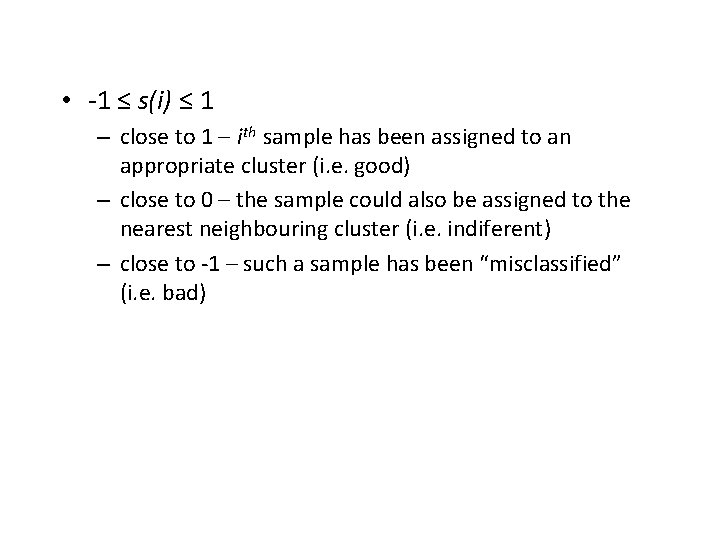
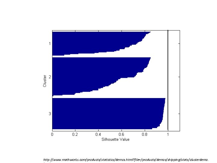
• -1 ≤ s(i) ≤ 1 – close to 1 – ith sample has been assigned to an appropriate cluster (i. e. good) – close to 0 – the sample could also be assigned to the nearest neighbouring cluster (i. e. indiferent) – close to -1 – such a sample has been “misclassified” (i. e. bad)

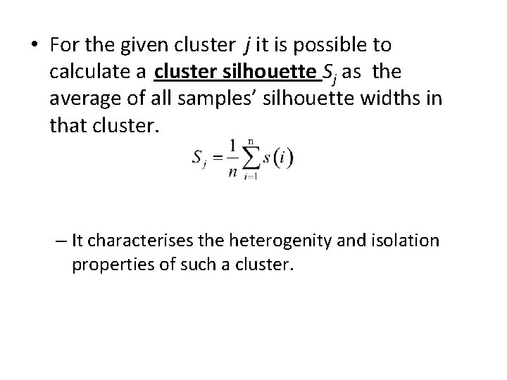
• For the given cluster j it is possible to calculate a cluster silhouette Sj as the average of all samples’ silhouette widths in that cluster. – It characterises the heterogenity and isolation properties of such a cluster.

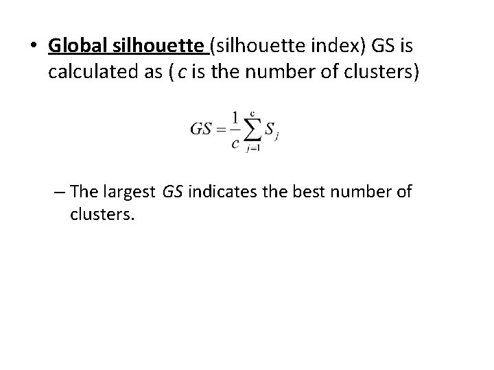
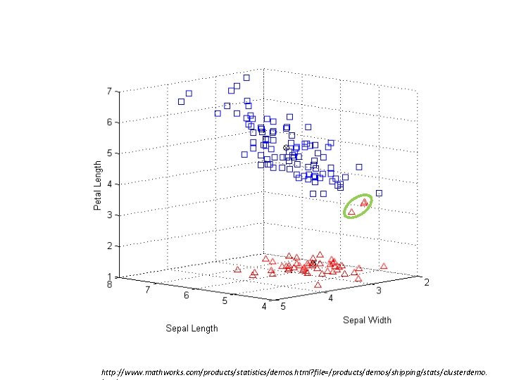
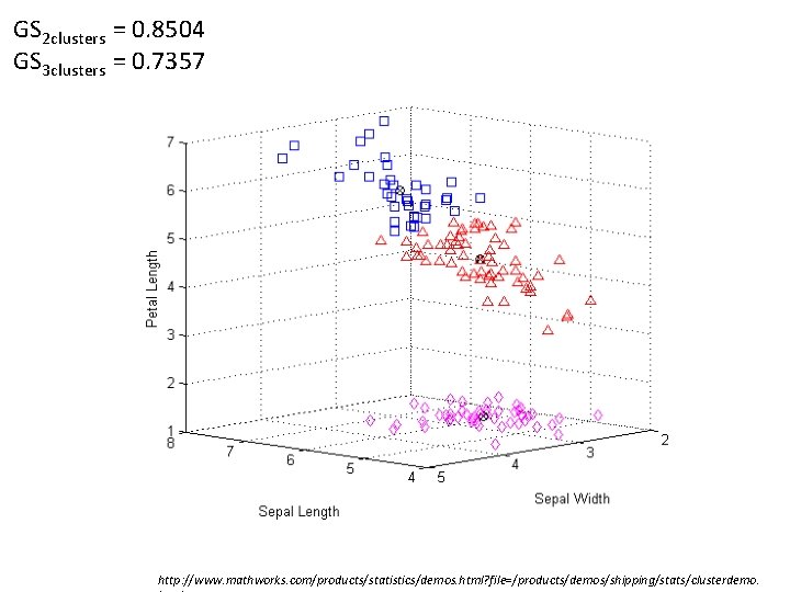
• Global silhouette (silhouette index) GS is calculated as ( c is the number of clusters) – The largest GS indicates the best number of clusters.

Iris data k-means – silhouette http: //www. mathworks. com/products/statistics/demos. html? file=/products/demos/shipping/stats/clusterdemo.

http: //www. mathworks. com/products/statistics/demos. html? file=/products/demos/shipping/stats/clusterdemo.

http: //www. mathworks. com/products/statistics/demos. html? file=/products/demos/shipping/stats/clusterdemo.

GS 2 clusters = 0. 8504 GS 3 clusters = 0. 7357 http: //www. mathworks. com/products/statistics/demos. html? file=/products/demos/shipping/stats/clusterdemo.