Last lecture summary Standard normal distribution Zdistribution Ztable

Last lecture summary • Standard normal distribution, Z-distribution • Z-table • lognormal distribution, geometric mean

Z-table What is the proportion less than the point with the Z-score -2, 75? Nice applet: http: //www. mathsisfun. com/data/standard-normal-distribution-table. html

How normal is normal? Checking normality 1. Eyball histograms 2. Eyball QQ plots 3. There are tests http: //www. nate-miller. org/blog/how-normal-is-normal-a-q-q-plot-approach

QQ plot • Q stands for ‘quantile’. Quantiles are values taken at regular intervals from the data. The 2 -quantile is called the median, the 3 -quantiles are called terciles, the 4 -quantiles are called quartiles (deciles, percentiles).

How to interpret QQ plot

How to interpret QQ plot no outlier

http: //www. nate-miller. org/blog/how-normal-is-normal-a-q-q-plot-approach

Typical normal QQ plot http: //emp. byui. edu/Brown. D/Stats-intro/dscrptv/graphs/qq-plot_egs. htm

QQ plot of left-skewed distribution http: //emp. byui. edu/Brown. D/Stats-intro/dscrptv/graphs/qq-plot_egs. htm

QQ plot of right-skewed distribution http: //emp. byui. edu/Brown. D/Stats-intro/dscrptv/graphs/qq-plot_egs. htm

SAMPLING DISTRIBUTIONS výběrová rozdělení

Histogram

Sampling distribution of sample mean • výběrové rozdělení výběrového průměru

Sweet demonstration of the sampling distribution of the mean

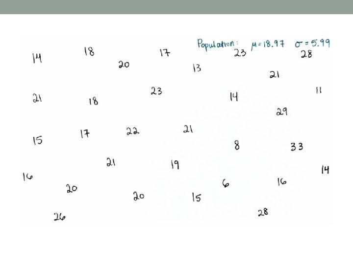
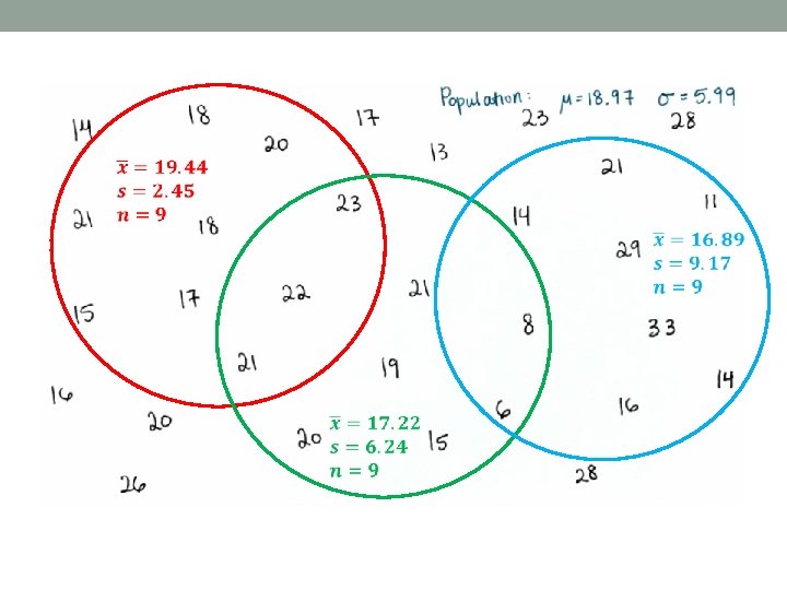
Data 2013 Population: 6, 4, 5, 3, 10, 3, 5, 3, 6, 5, 4, 8, 7, 2, 8, 5, 4, 0 20 samples (n=3) and their averages 1. 10 3 5 … 6. 0 2. 3 3 4 … 3. 3 3. 4 4 8 … 5. 3 4. 4 3 8 … 5. 0 5. 5 5 6 … 5. 3 6. 6 8 7 … 7. 0 7. 3 8 8 … 6. 3 8. 6 8 4 … 6. 0 9. 8 8 4 … 6. 7 10. 5 3 4… 4. 0 11. 2 10 8… 6. 7 12. 3 4 5 … 4. 0 13. 5 6 5 … 5. 3 14. 8 6 4 … 6. 0 15. 4 8 4 … 5. 3 16. 5 8 5 … 6. 0 17. 4 4 3 … 3. 7 18. 8 8 4… 6. 7 19. 8 4 5… 5. 7 20. 3 0 7… 3. 3 http: //blue-lover. blog. cz/1106/lentilky

Data 2014 Population: 3, 2, 3, 1, 2, 6, 5, 5, 4, 3, 5, 5, 6, 3, 2, 4, 4, 3, 1, 5 20 samples (n=3) and their averages 1. 5 1 4 … 3. 3 2. 3 1 1 … 1. 7 3. 6 6 5 … 5. 7 4. 3 5 4 … 4. 0 5. 4 1 4 … 3. 0 6. 5 1 3 … 3. 0 7. 2 5 4 … 3. 7 8. 5 5 1 … 3. 7 9. 3 3 5 … 3. 7 10. 5 2 3 … 3. 3 11. 5 3 4 … 4. 0 12. 3 4 6 … 4. 3 13. 2 5 5 … 4. 0 14. 5 6 1 … 4. 0 15. 2 2 5 … 3. 0 16. 5 3 6 … 4. 7 17. 1 5 3 … 3. 0 18. 5 5 5 … 5. 0 19. 3 5 4 … 4. 0 20. 3 3 6 … 4. 0 http: //blue-lover. blog. cz/1106/lentilky

Sampling distribution, n = 3 Plot exact sampling distribution sample_size <- 3 data. set 2014 <- c(3, 2, 3, 1, 2, 6, 5, 5, 4, 3, 5, 5, 6, 3, 2, 4, 4, 3, 1, 5) samps <- combn(data. set 2014, sample_size) xbars <- col. Means(samps) barplot(table(xbars))

Sampling distribution, n = 3 •

Sampling distribution, n = 3

Sampling distribution, n = 5

Central limit theorem •

Quiz • As the sample size increases, the standard error • increases • decreases • As the sample size increases, the shape of the sampling distribution gets • skinnier • wider

Another data 1, 1, 1, 2, 2, 2, 3, 3, 4, 4, 4, 5, 5, 6, 7, 7, 8, 8, 8, 9, 9, 10, 10, 10, 11, 11, 11

Sampling distribution n=2

Sampling distribution n=4

Sampling distribution n=6

Sampling distribution n=8

Sampling distribution applet parent distribution sample data sampling distributions of selected statistics http: //onlinestatbook. com/stat_sim/sampling_dist/index. html