Last lecture summary Probability model probability model Formulas

Last lecture summary

Probability model • probability model – Formulas to calculate probabilities – Determine average outcomes – Figure out the amount of variability in data • fundamental parts of probability model: – random variable – probability distribution

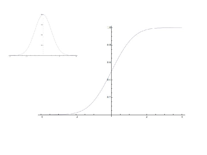
Probability distribution • Function assigning a probability P(X) to the event that X was observed. • Dicrete case – probability mass function, PMF, pravděpodobnostní funkce • Continuous case – probability density function, pdf, hustota pravděpodobnosti

from Probability for Dummies, D. Rumsey

Distribution function • Cumulative distribution function (cdf) F(a) – probability that X is less or equal to the given value a

cdf is defined on all values from -Inf to +Inf F(6) … less than 7 from Probability for Dummies, D. Rumsey

Expected value, variance • Expected value E(X) – long-term average outcome of a random variable – It is a mean (average) of X • Variance (rozptyl) V(X) – amount of variability in data – Standard deviation (směrodatná odchylka) – square root of variance

Statistical jargon • population (census) vs. sample • parameter (population) vs. statistic (sample) • bias

Summarizing numerical data • where the center is (i. e. what’s a typical value) • how spread the data are • where certain milestones are

Center •

New stuff

Accounting for variation • variability always exist in data, e. g. income of household varies household to household, year to year, country to country • the most commonly used measure of variability is the standard deviation s (směrodatná odchylka) • it represents a typical distance from any point in the data set to the center – it’s roughly the average distance from the center (from the average value of data)

• small stdev – data are close to the middle of data set • When interpreting stdev, watch for – units – stdev of 2 years is equivalent to a stdev of 24 months – the value of the mean – if average is 5. 2 and stdev is 3. 4, it’s a lot of variability, relatively speaking. But if the average is 25. 6, stdev of 3. 4 is comparably smaller. • Standard deviation is not a robust statistic. – Median Absolute Deviation (MAD) (mediánová absolutní odchylka) – For observations x 1, x 2, . . . , xn, with median m, the MAD is the median of the differences |x 1−m|, |x 2−m|, . . . , |xn−m|.

• For normal (Gauss) distribution there exist nice empirical rule that helps to interpret the stdev. – about 68% of data lies lie within one stdev of either side of the mean, 95% within 2σ, 99, 7% within 3σ – More on that later. • Standard deviation is not reported very often in the media. And this is a big mistake ! – Average salary at VSCHT is 38 000, - CZK. Wow, that’s great! However, s=10 000, -. Hmm, based on the empirical rule you can make anywhere between 18 000, - and 58 000, - (that’s where 95% of data lie).

Percentiles • If doing some test (e. g. TOEFL), along with your score you want to know what the score means relative to the others who took the same exam with you. • Percentile is the percentage of individuals in the data set who are below you. • If you’re at the 90 th percentile, 90% of people scored lower than you, 10% higher. • Some have special names: – 1 st quartile (Q 1) – 25% – 2 nd quartile (Q 2) – 50% (i. e. median) – 3 rd quatile (Q 3) – 75%

Gauss distribution • also called normal distribution • continuous distribution • many variables have this distribution (e. g. heights, weights, lifetimes of products, …) • bell-shaped (i. e. there is a big group of individuals in the middle with fewer and fewer individuals on the sides) • because of the symmetry, mean μ and meadian are the same

1σ 1σ mean μ N(μ, σ), in this case N(1000, 20) from Statistics for Dummies, D. Rumsey

• This is empirical rule ! • About 68% of values lie within 1σ. • We will see later how to calculate these percentages exactly. • The rule does not apply if the distribution does not have a bell shape. from Statistics for Dummies, D. Rumsey

Standard score • Suppose that organic chemistry student Uhlík took a test for certification to become an organic chemist with the score of 235. • All you know is that the scores for this test had a normal distribution. • Is Uhlík's score a good one, a bad one, or is it just a middle-of-the-road result? • You can't answer this question without a measure of where Uhlík stands among the other people who took the test.

• You can determine the relative standing for Uhlík's test score (235) in a number of ways - some are better than others. 1. look at the score in terms of the total points possible (300) – not very informative 2. compare his result to the average value (250) – at this point we know Uhlík scored 15 below the average – But what does the difference of 15 means in this situation? 3. look at the σ – σ = 5. . . 15 points is 3σ, which is a lot (how many of other test takers scored lower than him? ) – σ = 15 … scores are much more variable (how many of other test takers scored lower than him in this case? )

• So the relative standing of any score apparently depends on the standard deviation (score didn’t change from one scenario to another, but the interpretation did). • To interpret the relative standing of any value on a normal distribution use standard score (z -score). (standardizované, z-skóre) • It is a standardized version of the original score; it represents the number of standard deviations above/below the mean.

• Almost all (99. 7%) z-scores fall between values -3 and +3. • negative – value is below the mean • positive – value is above the mean • 0 – value is mean • z-scores have special normal distribution with mean 0 and σ 1 (N(0, 1)) call standard normal distribution or zdistribution (standardizované normální rozdělení)

• The standard scores have the universal interpretation which makes them great. • To interpret standard scores, you don’t need to know the original scores, their mean or their standard deviation. from Statistics for Dummies, D. Rumsey

Variability in sample results • If you are not able to conduct census, you sample from the population and you calculate the sample statistic (e. g. mean) for this particular sample. • If you created different sample from the same population, the statistic would be slightly different. • Because sample results vary from sample to sample, the statistic (e. g. mean) should be reported not as one value, but as interval (or as famous ±).

Standard error • Variability in sample mean is measured in terms of standard errors (střední chyba odhadu, směrodatná chyba). • Standard error is the same concept as standard deviation – both represent a typical distance from the mean. • But they differ in their nature. – The original population values deviate due to natural phenomena (people have different heights). – Sample means vary because of the error that occurs in not doing a census and being able to only take samples.

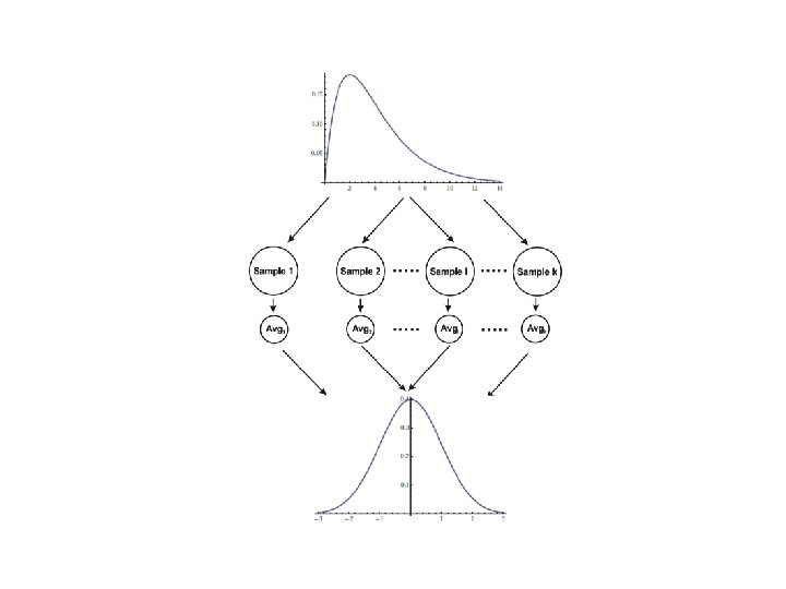
Sampling distribution • Listing of all values mean can take + how often these values occur is called sampling distribution (výběrové rozdělení) of the sample mean. • It has shape, center, and the measure of variability (standard error). • If the samples are large enough, the sampling distribution of the mean is normal, regardless what the distribution of the sample data is! • This is called the central limit theorem (CLT).

• Because the sampling distribution of sample mean is normal, you can use empirical rule to get an idea how much a given sample result will vary: – about 68% of the sample means lie within 1 standard error – about 95% of the sample means lie within 2 standard error – about 99. 7% of the sample means lie within 3 standard error

• What does the empirical rule tell you about how much you can expect a given sample mean to vary? • Keep in mind that 95% of the sample means should lie within 2 standard errors of the population mean, and your job is to estimate the population mean. • So, if your estimate is actually a range including your sample mean plus or minus 2 standard errors, your estimate would be correct about 95% of the time.

• This type of result, involving a statistic plus or minus a certain number of standard errors, is called a confidence interval (interval spolehlivosti). The amount added or subtracted is called the margin of error. • And how do we obtain the mean of the distribution of sample means and the standard error?

• CLT knows the answer to that – The distribution of all possible sample means is approximately normal. – The larger the size n is, the closer the distribution is to the normal one (n ≥ 30 is large enough). – The mean of the distribution of sample means is also μ. – The standard error of the sample means is – The standard error decreases with increasing size of the sample. – Also, as the variability in the population increases, so does the variability in the sample mean.

• quick-and-dirty way (statistically incorrect) to get a rough idea of the margin of error (for categorical data !) just based on the sample size n • i. e. if your sample size is 1000, margin of error is 3% • That’s actually amazing, imagine you want to investigate the whole Czech population, but choosing (clever!) of 1000 people gives you error only in units of percents.