Last lecture summary Multilayer perceptron MLP the most

Last lecture summary

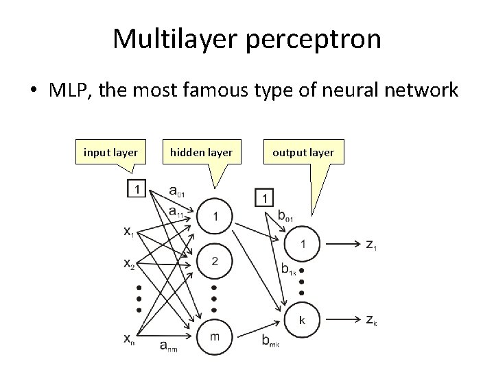
Multilayer perceptron • MLP, the most famous type of neural network input layer hidden layer output layer

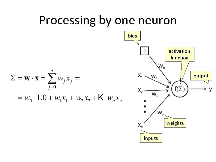
Processing by one neuron bias activation function output weights inputs

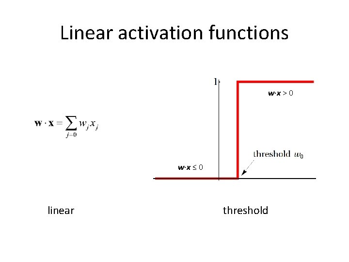
Linear activation functions w∙x > 0 w∙x ≤ 0 linear threshold

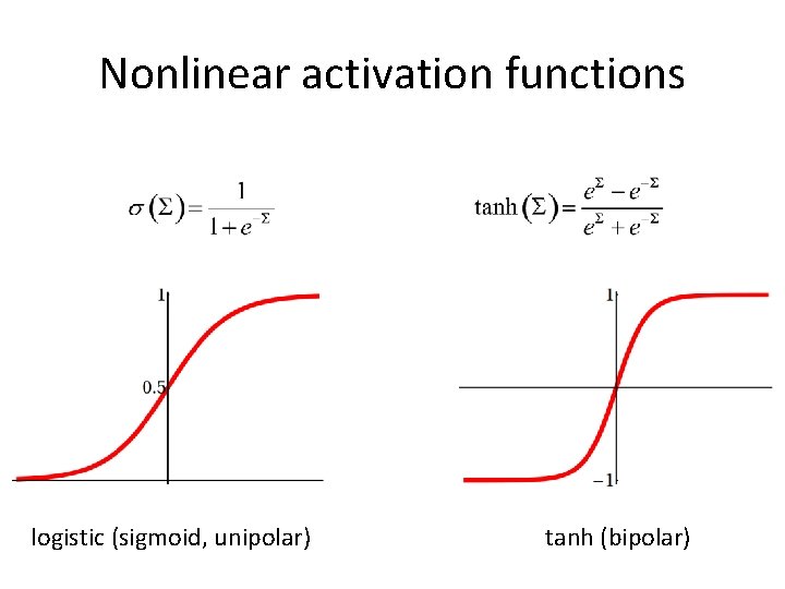
Nonlinear activation functions logistic (sigmoid, unipolar) tanh (bipolar)

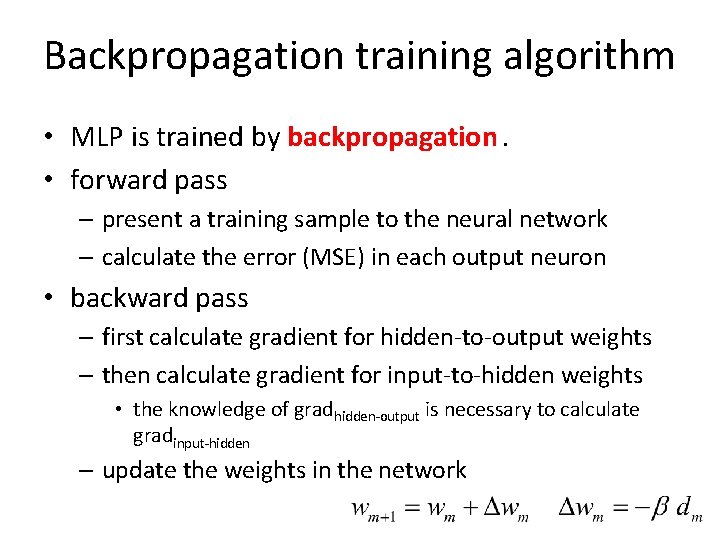
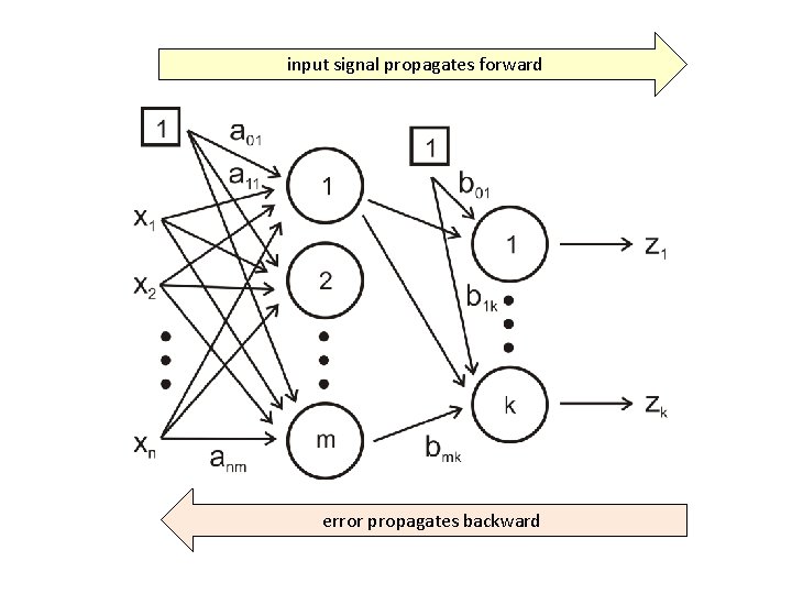
Backpropagation training algorithm • MLP is trained by backpropagation. • forward pass – present a training sample to the neural network – calculate the error (MSE) in each output neuron • backward pass – first calculate gradient for hidden-to-output weights – then calculate gradient for input-to-hidden weights • the knowledge of gradhidden-output is necessary to calculate gradinput-hidden – update the weights in the network

input signal propagates forward error propagates backward

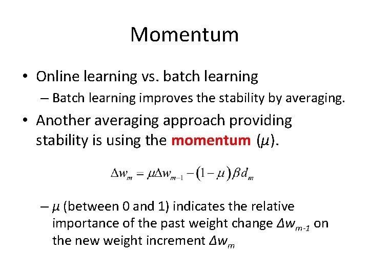
Momentum • Online learning vs. batch learning – Batch learning improves the stability by averaging. • Another averaging approach providing stability is using the momentum (μ). – μ (between 0 and 1) indicates the relative importance of the past weight change ∆wm-1 on the new weight increment ∆wm

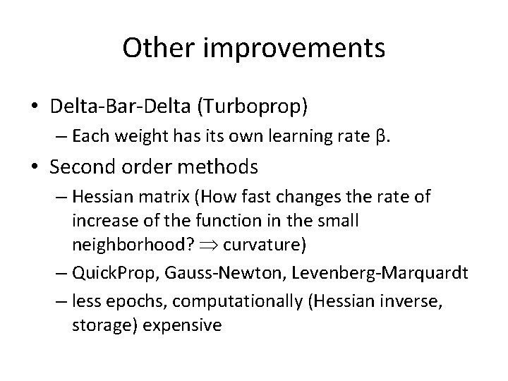
Other improvements • Delta-Bar-Delta (Turboprop) – Each weight has its own learning rate β. • Second order methods – Hessian matrix (How fast changes the rate of increase of the function in the small neighborhood? curvature) – Quick. Prop, Gauss-Newton, Levenberg-Marquardt – less epochs, computationally (Hessian inverse, storage) expensive

New stuff

Bias-variance • Just a small reminder • bias (lack of fit, undefitting) – model does not fit data enough, not enough flexible (too small number of parameters) • variance (overfitting) – model is too flexible (too much parameters), fits noise • bias-variance tradeoff – improving the generalization ability of the model (i. e. find the correct amount of flexibility)

• Parameters in MLP: weights • If you use one more hidden neuron, the number of weights increases by how much? – # input neurons + # output neurons • If MLP is used for regression task, be careful! • To use MLP statistically correctly, the number of degrees of freedoms (i. e. weights) can’t exceed the number of data points. – Compare to polynomial regression example from the 2 nd lecture

Improving generalization of MLP • Flexibility comes from hidden neurons. • Choose such a # of hidden neurons so neither undefitting, nor overfitting occurs. • Three most common approaches: – exhaustive search – early stopping – regularization

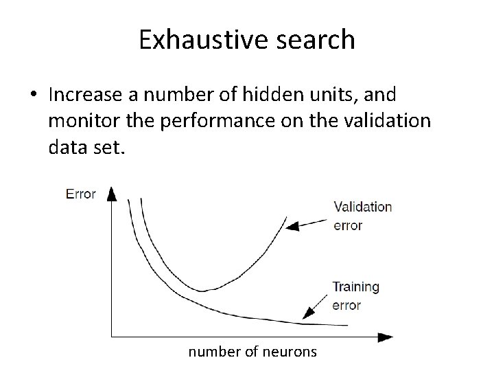
Exhaustive search • Increase a number of hidden units, and monitor the performance on the validation data set. number of neurons

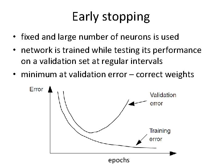
Early stopping • fixed and large number of neurons is used • network is trained while testing its performance on a validation set at regular intervals • minimum at validation error – correct weights epochs

Weight decay • Idea: keep the growth of weights to a minimum in such a way that non-important weights are pulled toward zero • Only the important weights are allowed to grow, others are forced to decay • regularization

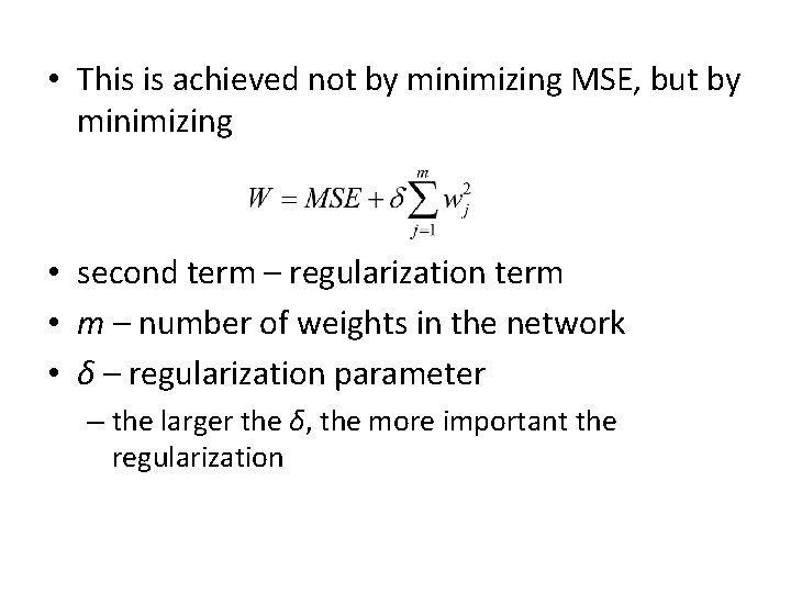
• This is achieved not by minimizing MSE, but by minimizing • second term – regularization term • m – number of weights in the network • δ – regularization parameter – the larger the δ, the more important the regularization

Network pruning • Both early stopping and weight decay use all weights in the NN. They do not reduce the complexity of the model. • Network pruning – reduce complexity by keeping only essential weights/neurons. • Several pruning approaches, e. g. – optimal brain damage (OBD) – optimal brain surgeon (OBS) – optimal cell damage (OCD)

Radial Basis Function Networks

Radial Basis Function (RBF) Network • Becoming an increasingly popular neural network. • Is probably the main rival to the MLP. • Completely different approach by viewing the design of a neural network as an approximation problem in high-dimensional space. • Uses radial functions as activation function.

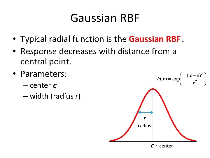
Gaussian RBF • Typical radial function is the Gaussian RBF. • Response decreases with distance from a central point. • Parameters: – center c – width (radius r) r radius c - center

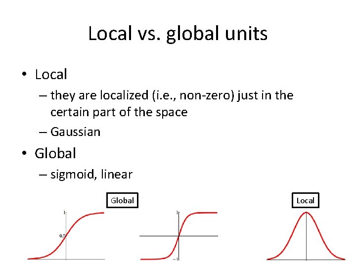
Local vs. global units • Local – they are localized (i. e. , non-zero) just in the certain part of the space – Gaussian • Global – sigmoid, linear Global Local

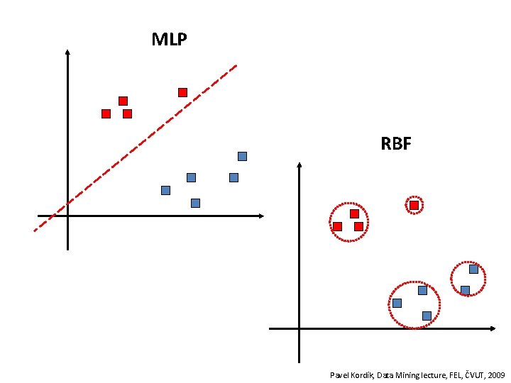
MLP RBF Pavel Kordík, Data Mining lecture, FEL, ČVUT, 2009

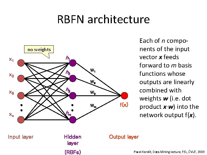
RBFN architecture Each of n components of the input vector x feeds forward to m basis functions whose outputs are linearly combined with weights w (i. e. dot product x∙w) into the network output f(x). no weights x 1 h 1 x 2 h 2 W 1 W 2 x 3 h 3 Wm xn hm Input layer Hidden layer (RBFs) f(x) Output layer Pavel Kordík, Data Mining lecture, FEL, ČVUT, 2009

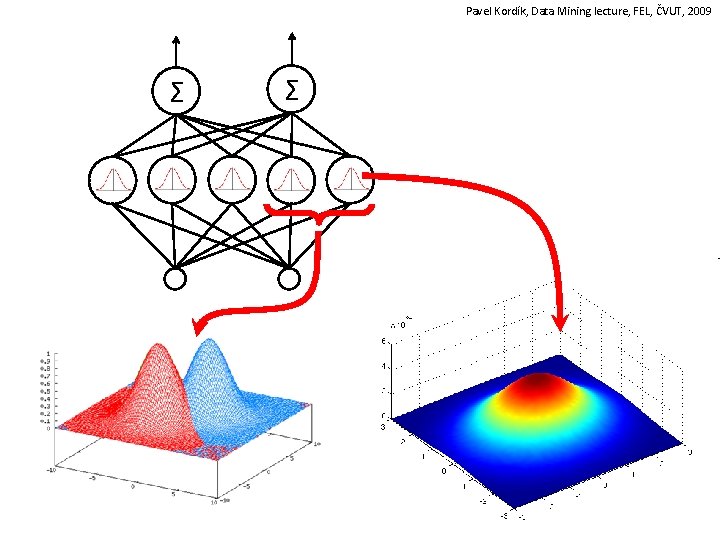
Pavel Kordík, Data Mining lecture, FEL, ČVUT, 2009 Σ Σ

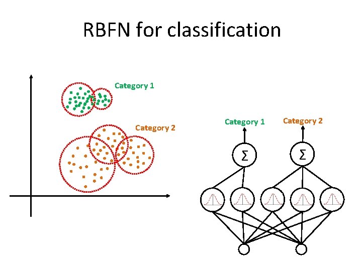
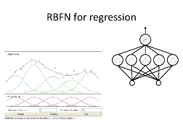
• The basic architecture for a RBF is a 3 -layer network. • The input layer is simply a fan-out layer and does no processing. • The hidden layer performs a non-linear mapping from the input space into a (usually) higher dimensional space in which the patterns become linearly separable. • The output layer performs a simple weighted sum (i. e. w∙x). – If the RBFN is used for regression then this output is fine. – However, if pattern classification is required, then a hardlimiter or sigmoid function could be placed on the output neurons to give 0/1 output values

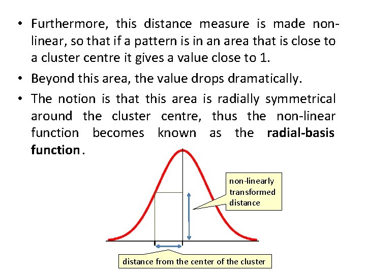
Clustering • The unique feature of the RBF network is the process performed in the hidden layer. • The idea is that the patterns in the input space form clusters. • If the centres of these clusters are known, then the distance from the cluster centre can be measured.

• Furthermore, this distance measure is made nonlinear, so that if a pattern is in an area that is close to a cluster centre it gives a value close to 1. • Beyond this area, the value drops dramatically. • The notion is that this area is radially symmetrical around the cluster centre, thus the non-linear function becomes known as the radial-basis function. non-linearly transformed distance from the center of the cluster

RBFN for classification Category 1 Category 2 Σ Σ

RBFN for regression

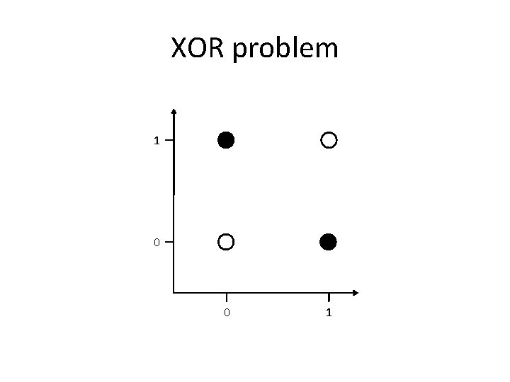
XOR problem 1 0 0 1

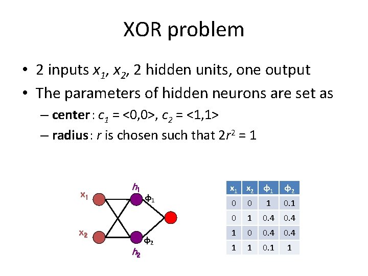
XOR problem • 2 inputs x 1, x 2, 2 hidden units, one output • The parameters of hidden neurons are set as – center: c 1 = <0, 0>, c 2 = <1, 1> – radius: r is chosen such that 2 r 2 = 1 x 1 h 1 x 2 h 2 φ1 φ2 x 1 x 2 φ1 φ2 0 0 1 0. 4 0. 4 1 0 0. 4 1 1 0. 1 1

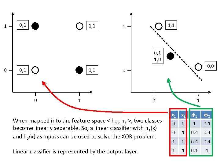
1 0, 1 1, 1 1 0, 1 1, 0 0 0, 0 0 1 When mapped into the feature space < h 1 , h 2 >, two classes become linearly separable. So, a linear classifier with h 1(x) and h 2(x) as inputs can be used to solve the XOR problem. Linear classifier is represented by the output layer. 1 0 x 1 x 2 φ1 φ2 0 0 1 0. 4 0. 4 1 0 0. 4 1 1 0. 1 1

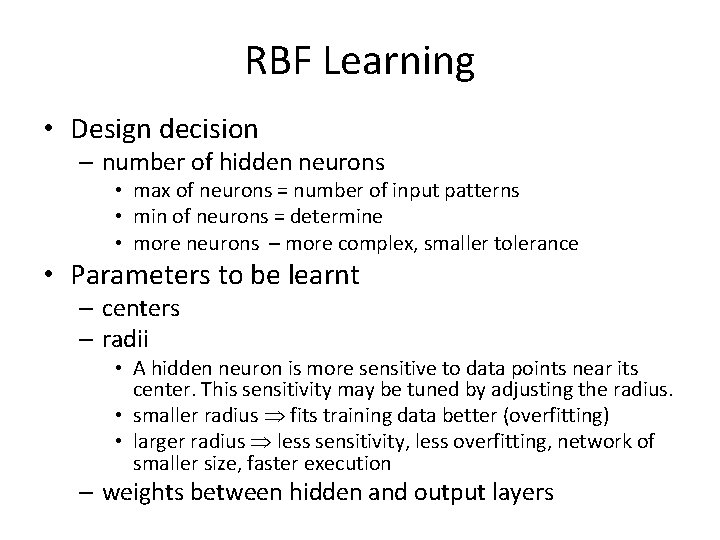
RBF Learning • Design decision – number of hidden neurons • max of neurons = number of input patterns • min of neurons = determine • more neurons – more complex, smaller tolerance • Parameters to be learnt – centers – radii • A hidden neuron is more sensitive to data points near its center. This sensitivity may be tuned by adjusting the radius. • smaller radius fits training data better (overfitting) • larger radius less sensitivity, less overfitting, network of smaller size, faster execution – weights between hidden and output layers

• Learning can be divide in two independent tasks: 1. Center and radii determination 2. Learning of output layer weights • Learning strategies for RBF parameters 1. Sample center position randomly from the training data 2. Self-organized selection of centers 3. Both layers are learnt using supervised learning

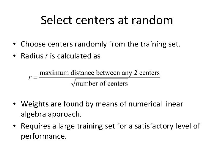
Select centers at random • Choose centers randomly from the training set. • Radius r is calculated as • Weights are found by means of numerical linear algebra approach. • Requires a large training set for a satisfactory level of performance.

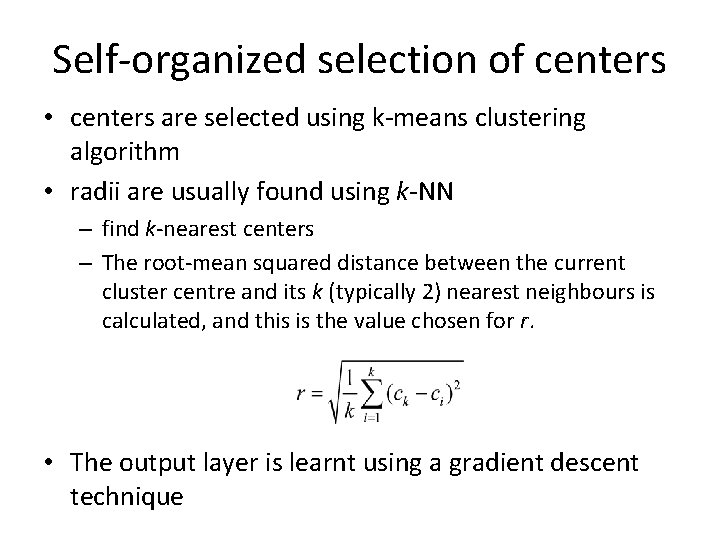
Self-organized selection of centers • centers are selected using k-means clustering algorithm • radii are usually found using k-NN – find k-nearest centers – The root-mean squared distance between the current cluster centre and its k (typically 2) nearest neighbours is calculated, and this is the value chosen for r. • The output layer is learnt using a gradient descent technique

Supervised learning • Supervised learning of all parameters (centers, radii, weights) using gradient descent. • Mathematical formulas for updating all of these parameters. They are not shown here, I don’t want to scare you more than necessary.

RBFN and MLP • RBFN trains faster than a MLP • Although the RBFN is quick to train, it is slower in retrieving than a MLP. • RBFNs are essentially well established statistical techniques being presented as neural networks. Learning mechanisms in statistical neural networks are not biologically plausible. • RBFN can give “I don’t know” answer. • RBFN construct local approximations to nonlinear I/O mapping. MLP construct global approximations to non-linear I/O mapping.