Laser Interferometer Space Antenna LISA Simulating the WDWD

Laser Interferometer Space Antenna (LISA) Simulating the WD-WD galactic background in the LISA data Massimo Tinto JPL - CIT http: //science. jpl. nasa. gov/Astrophysics/index. cfm J. Edlund, M. Tinto, A. Krolak, and G. Nelemans, Phys. Rev. D. 71, 122003 (2005) GSFC JPL Isola d’Elba, Italy, 05/28 – 06/01 2006

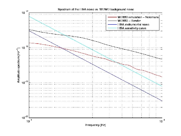
Motivations • Need for a numerical description of the WD -WD background as it will be observed in the LISA data. – Assess its magnitude in the various TDI combinations – Quantify the effects of the LISA motion around the Sun. – Test the effectiveness of various data analysis techniques for removing it from the LISA data. D. Hils & P. Bender, R. F. Webbink, Ap. J. 360, 75 (1990) D. Hils & P. Bender, CQG, 1439 (1997)

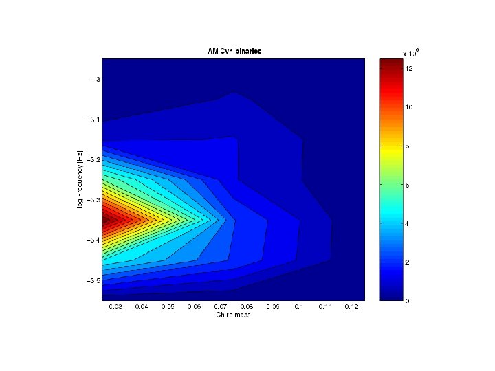
Parameters Distribution Each GW signal depends on 8 parameters: (Mc, w, l, b, i, y, f 0, D) • The overall P. D. F can be assumed to have the following form: P(Mc, w, l, b, i, y, f 0, D) = P 1(Mc, w) P 2(y) P 3(i) P 4(l, b, D) P 5(f 0)

WD-WD Binaries Distribution G. Nelemans, L. R. Yungelson, and S. F. Portegies-Zwart, A&A. , 375, 890, (2001) G. Nelemans, L. R. Yungelson, and S. F. Portegies-Zwart, Mon. Not. Roy. Astron. Soc. , 349, 181 (2004)

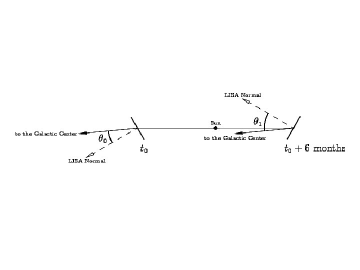
Geometry To the Autumn Equinox To the Galactic Center

Numerical Simulation • To generate, in the time-domain, 1 year of the X-response to 1 WD -WD signal takes ~ 10 seconds on a 3. 2 GHz P 4 CPU (an optimized code can make it in 1 second. ) • For 2. 6 x 107 sources it would take an unacceptably long time! • We have derived an analytic expression of the infinite Fourier transform of the signal from a galactic WD-WD binary as seen in any TDI combination. • Our simulation relies on the convolution of this expression with a properly selected window function. • We have compared the final time-domain expression of the response obtained using our Fourier-based analytic formula against the time-domain computed expression and found perfect agreement. • Using our algorithm the CPU time/source => ~ 0. 1 seconds! • For performing our simulation we relied on the JPL Supercomputer (3 days of processing!)

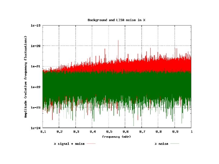
Long-Wavelength Expansion • Since the contribution of the background to the LISA data is in the low-part of the frequency band, i. e. in the regime where x = 2 p f L/c <<1, we have Taylor-expanded the TDI responses for each individual signal. • Care must be taken in selecting the order of the Taylor expansion in x for any considered TDI response. • We have simulated the response of the Xcombination to the WD-WD background.

L. W. E. Accuracy

N. Seto, Phys. Rev. D, 69, 123005, (2004)

Cyclo. Stationarity • The motion of LISA around the Sun induces a AMFM modulation of the received signals. • In a statistical sense the WD-WD background should be regarded as a periodic function of time with period 1 year. • Since the autocorrelation will also be a periodic function of time, the background should no longer be treated as a stationary random process, but rather as a Cyclostationary process:

Cyclo. Stationarity…(cont. ) H. L. Hurd, IEEE Trans. Inf. Theory 35, 350, 1989

Cyclo. Stationarity…(cont. ) This implies that for r > 0 the cyclic spectra of yt coincide with those of ct , i. e. in principle they are not contaminated by the noise! In reality, possible non-stationarity of the noise will need to be accounted for (as always!)

Cyclostationarity and the WD-WD Inverse Problem • The cyclostationary spectra, gr (f), can be related to the distribution function of the WD-WD binaries. !!QUESTIONS!! • How could we solve for the WD-WD population distribution given these observables? • Is this the “optimal procedure” for solving the WDWD background inverse problem? • No matter what the optimal procedure will be, the astrophysical payoff will be very significant!!