LargeSignal Network Analyzer Technology An Overview and Examples

Large-Signal Network Analyzer Technology An Overview and Examples Copyright 2003 NMDG Engineering

Agenda l l l l Why “Large-Signal Network Analysis” is needed Large-Signal Network Analysis The Large-Signal Network Analyzer Calibration State of the art and evolution Application Examples Conclusions 2 Certain slides are with permission from Agilent Technologies

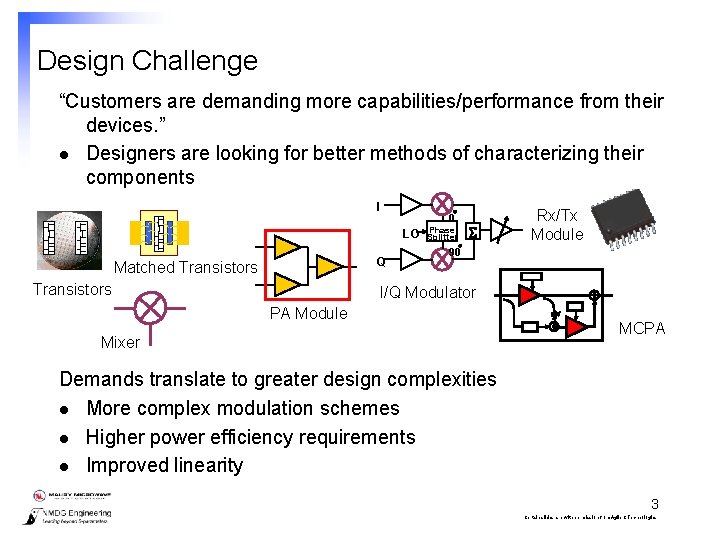
Design Challenge “Customers are demanding more capabilities/performance from their devices. ” l Designers are looking for better methods of characterizing their components I 0 LO Q Matched Transistors Phase Splitter S Rx/Tx Module 90 I/Q Modulator PA Module Mixer MCPA Demands translate to greater design complexities l More complex modulation schemes l Higher power efficiency requirements l Improved linearity 3 Certain slides are with permission from Agilent Technologies

Why can’t I predict component performance better? Existing tools are insufficient l Network analyzers analyze component behavior but only the small-signals (linear) behavior accurately l Signal analyzers evaluate partial properties of signals interacting with the test device, they do not analyze the component behavior while interacting with the (measurement) environment To understand problems / defects faster To do more complete tests l Need more realistic test conditions l Need for a network analyzer approach in large-signal environments 4 Certain slides are with permission from Agilent Technologies

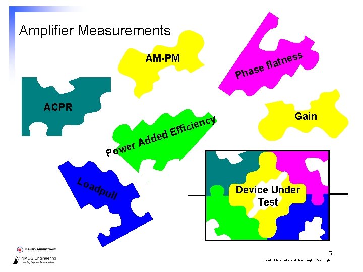
Amplifier Measurements es n t a l ef AM-PM s s Pha ACPR cy n e i c Gain fi P Loa dpu l Ad r e ow l Ef d e d Device Under Test 5 Certain slides are with permission from Agilent Technologies

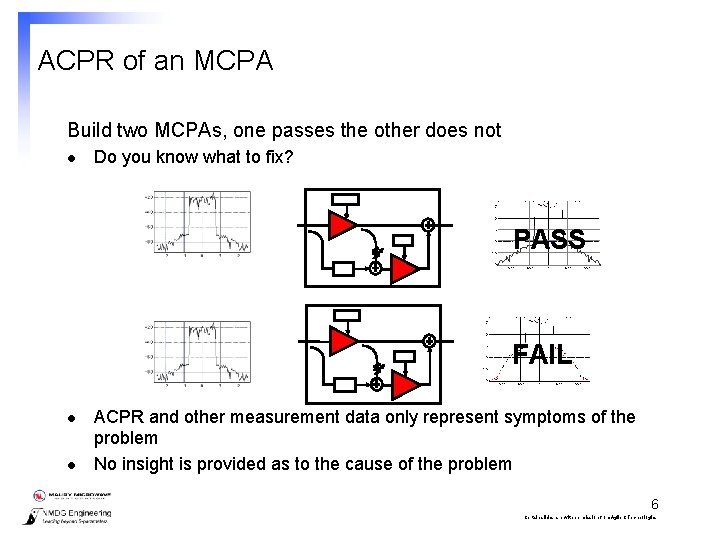
ACPR of an MCPA Build two MCPAs, one passes the other does not l Do you know what to fix? PASS FAIL l l ACPR and other measurement data only represent symptoms of the problem No insight is provided as to the cause of the problem 6 Certain slides are with permission from Agilent Technologies

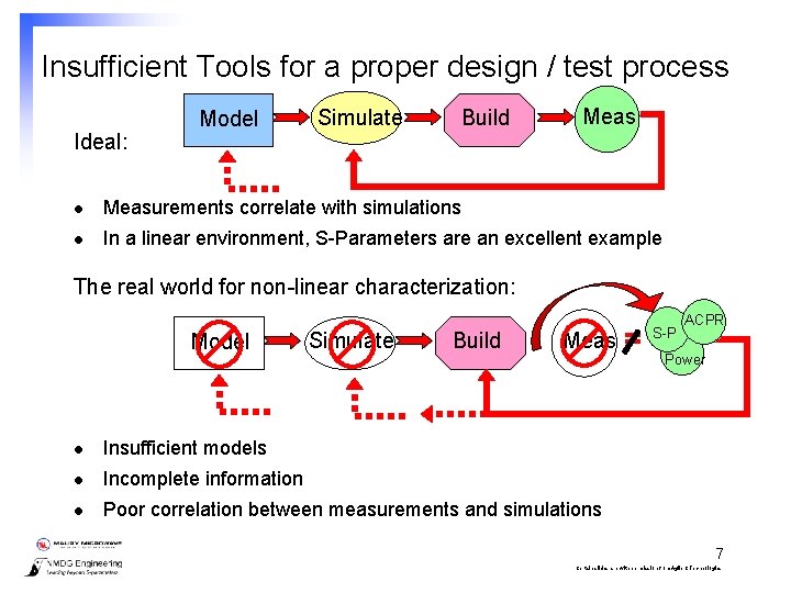
Insufficient Tools for a proper design / test process Ideal: Model Simulate Build Meas l Measurements correlate with simulations l In a linear environment, S-Parameters are an excellent example The real world for non-linear characterization: Model Simulate Build Meas l Insufficient models l Incomplete information l Poor correlation between measurements and simulations = S-P ACPR Power 7 Certain slides are with permission from Agilent Technologies

Results l l l Cut-and-try engineering (designers “imagineer” fixes) Design verification consumes 2/3 rds of development time Time-to-market delays Unpredictable design processes Time consuming tuning and measurement requirements 8 Certain slides are with permission from Agilent Technologies

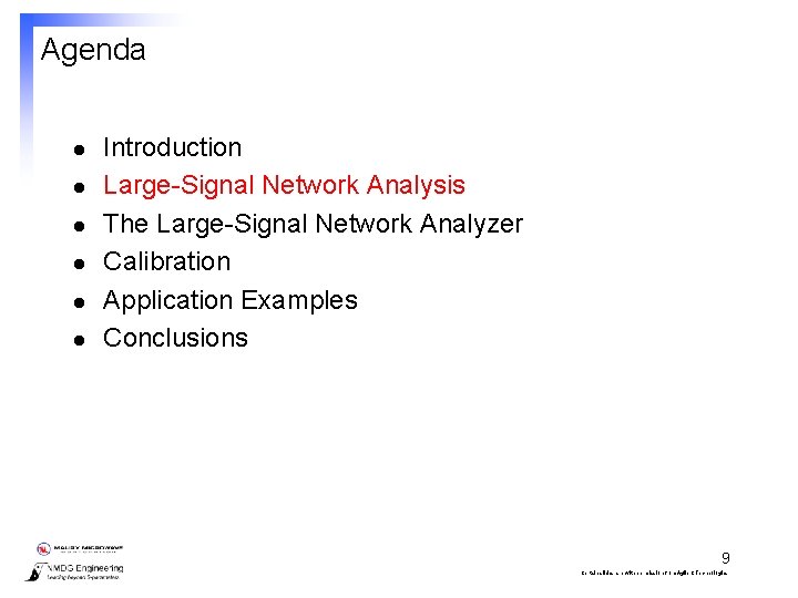
Agenda l l l Introduction Large-Signal Network Analysis The Large-Signal Network Analyzer Calibration Application Examples Conclusions 9 Certain slides are with permission from Agilent Technologies

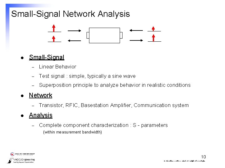
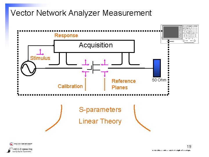
Small-Signal Network Analysis l l Small-Signal – Linear Behavior – Test signal : simple, typically a sine wave – Superposition principle to analyze behavior in realistic conditions Network – l Transistor, RFIC, Basestation Amplifier, Communication system Analysis – Complete component characterization : S - parameters (within measurement bandwidth) 10 Certain slides are with permission from Agilent Technologies

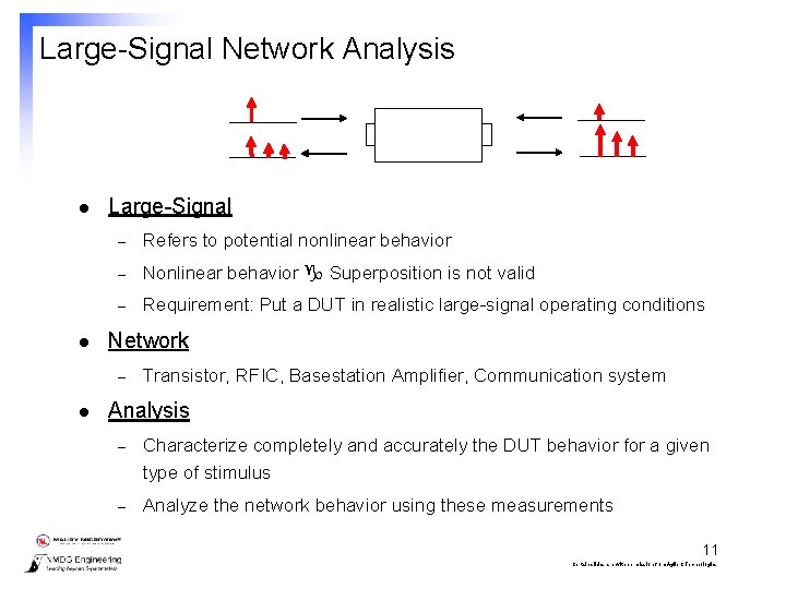
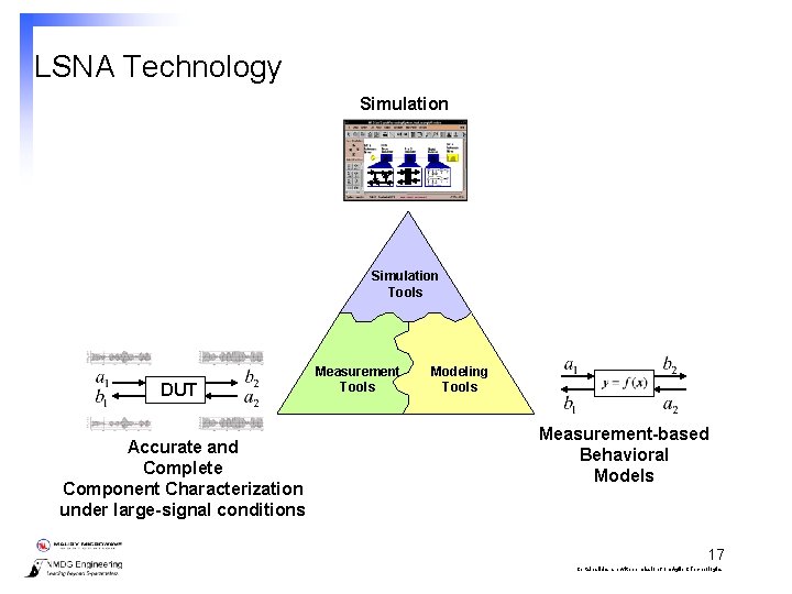
Large-Signal Network Analysis l l Large-Signal – Refers to potential nonlinear behavior – Nonlinear behavior Superposition is not valid – Requirement: Put a DUT in realistic large-signal operating conditions Network – l Transistor, RFIC, Basestation Amplifier, Communication system Analysis – Characterize completely and accurately the DUT behavior for a given type of stimulus – Analyze the network behavior using these measurements 11 Certain slides are with permission from Agilent Technologies

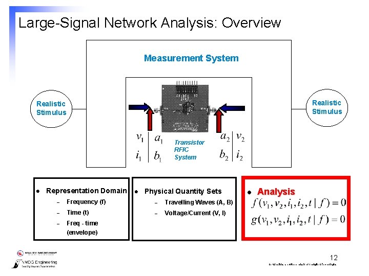
Large-Signal Network Analysis: Overview Measurement System Realistic Stimulus Transistor RFIC System l Representation Domain l Physical Quantity Sets – Frequency (f) – Travelling Waves (A, B) – Time (t) – Voltage/Current (V, I) – Freq - time (envelope) l Analysis 12 Certain slides are with permission from Agilent Technologies

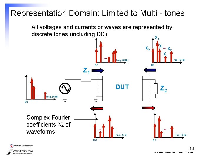
Representation Domain: Limited to Multi - tones All voltages and currents or waves are represented by discrete tones (including DC) X 1 Xi. . . X 0. . . Z 1 Xl Freq. (GHz) DC DC DUT. . . Xk Z 2 Freq. (GHz) DC Complex Fourier coefficients Xh of waveforms . . . Freq. (GHz) DC 13 Certain slides are with permission from Agilent Technologies

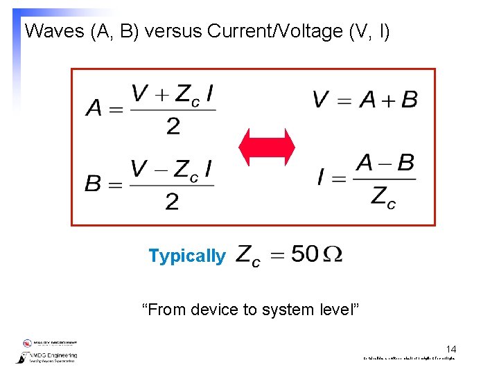
Waves (A, B) versus Current/Voltage (V, I) Typically “From device to system level” 14 Certain slides are with permission from Agilent Technologies

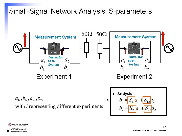
Small-Signal Network Analysis: S-parameters Measurement System Transistor RFIC System Experiment 2 Experiment 1 l Analysis 15 Certain slides are with permission from Agilent Technologies

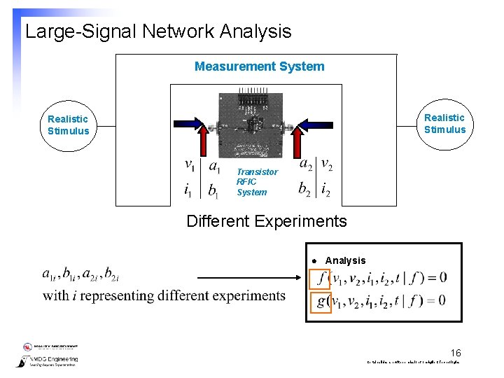
Large-Signal Network Analysis Measurement System Realistic Stimulus Transistor RFIC System Different Experiments l Analysis 16 Certain slides are with permission from Agilent Technologies

LSNA Technology Simulation Tools DUT Accurate and Complete Component Characterization under large-signal conditions Measurement Tools Modeling Tools Measurement-based Behavioral Models 17 Certain slides are with permission from Agilent Technologies

Agenda l l l Introduction Large-Signal Network Analysis The Large-Signal Network Analyzer Calibration Application Examples Conclusions 18 Certain slides are with permission from Agilent Technologies

Vector Network Analyzer Measurement Response Acquisition Stimulus Calibration Reference Planes 50 Ohm S-parameters Linear Theory 19 Certain slides are with permission from Agilent Technologies

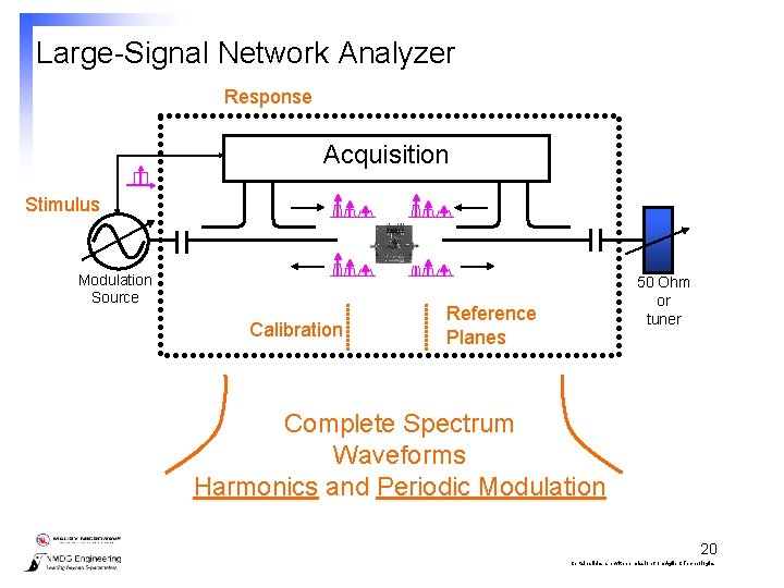
Large-Signal Network Analyzer Response Acquisition Stimulus Modulation Source Calibration 50 Ohm or tuner Reference Planes Complete Spectrum Waveforms Harmonics and Periodic Modulation 20 Certain slides are with permission from Agilent Technologies

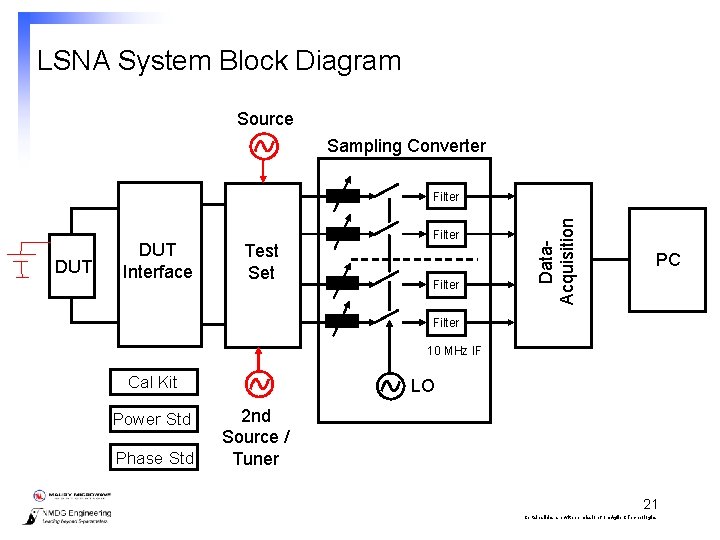
LSNA System Block Diagram Source Sampling Converter DUT Interface Test Set Filter Data. Acquisition Filter PC Filter 10 MHz IF Cal Kit Power Std Phase Std LO 2 nd Source / Tuner 21 Certain slides are with permission from Agilent Technologies

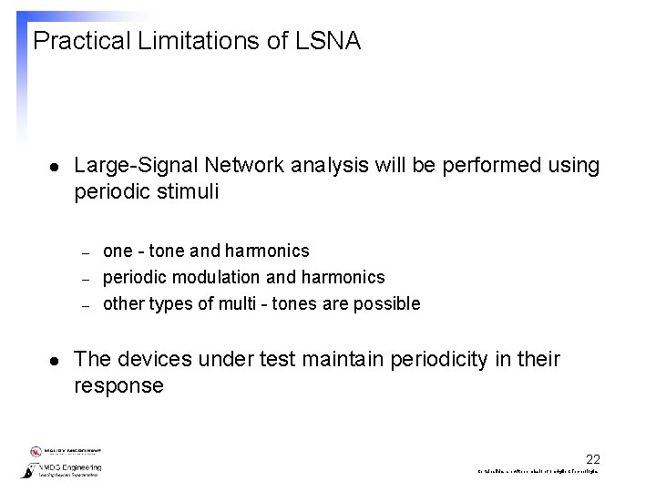
Practical Limitations of LSNA l Large-Signal Network analysis will be performed using periodic stimuli – – – l one - tone and harmonics periodic modulation and harmonics other types of multi - tones are possible The devices under test maintain periodicity in their response 22 Certain slides are with permission from Agilent Technologies

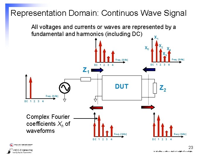
Representation Domain: Continuos Wave Signal All voltages and currents or waves are represented by a fundamental and harmonics (including DC) X 1 X 0 X 2 X 3 X 4 Freq. (GHz) Z 1 DC 1 2 3 4 DUT 4 Z 2 Freq. (GHz) DC 1 2 3 4 Complex Fourier coefficients Xh of waveforms Freq. (GHz) DC 1 2 3 4 23 Certain slides are with permission from Agilent Technologies

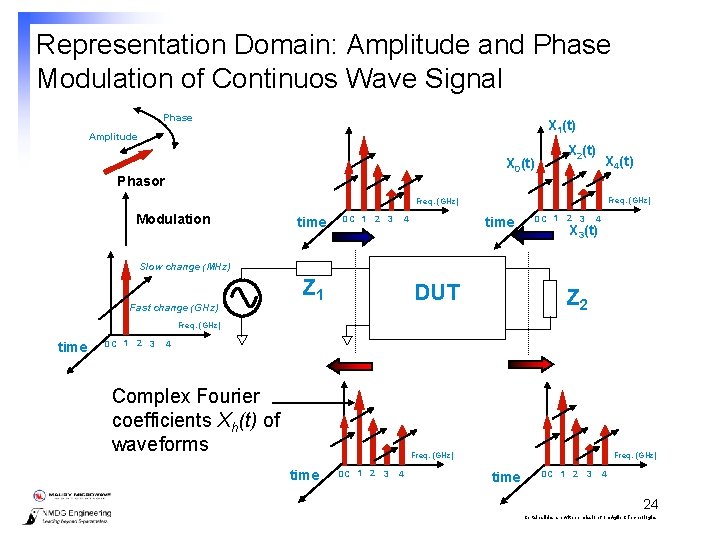
Representation Domain: Amplitude and Phase Modulation of Continuos Wave Signal Phase X 1(t) Amplitude X 0(t) Phasor X 2(t) X 4(t) Freq. (GHz) Modulation time DC 1 2 3 4 X 3(t) Slow change (MHz) Fast change (GHz) Z 1 DUT Z 2 Freq. (GHz) time DC 1 2 3 4 Complex Fourier coefficients Xh(t) of waveforms Freq. (GHz) time DC 1 2 3 4 24 Certain slides are with permission from Agilent Technologies

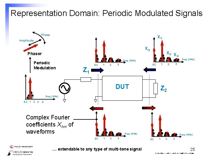
Representation Domain: Periodic Modulated Signals Phase X 1 i Amplitude X 0 i Phasor Periodic Modulation X 2 i X 3 i Freq. (GHz) Z 1 DC 1 2 DUT 3 2 1 DC 3 Z 2 Freq. (GHz) DC 1 2 3 4 Complex Fourier coefficients Xhm of waveforms Freq. (GHz) DC 1 2 3 … extendable to any type of multi-tone signal Freq. (GHz) DC 1 2 3 25 Certain slides are with permission from Agilent Technologies

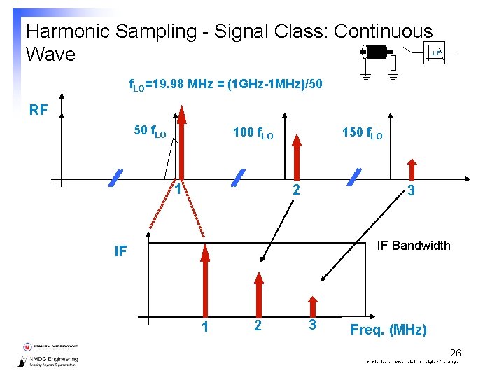
Harmonic Sampling - Signal Class: Continuous Wave LP f. LO=19. 98 MHz = (1 GHz-1 MHz)/50 RF 50 f. LO 100 f. LO 1 150 f. LO 2 3 IF Bandwidth IF 1 2 3 Freq. (MHz) 26 Certain slides are with permission from Agilent Technologies

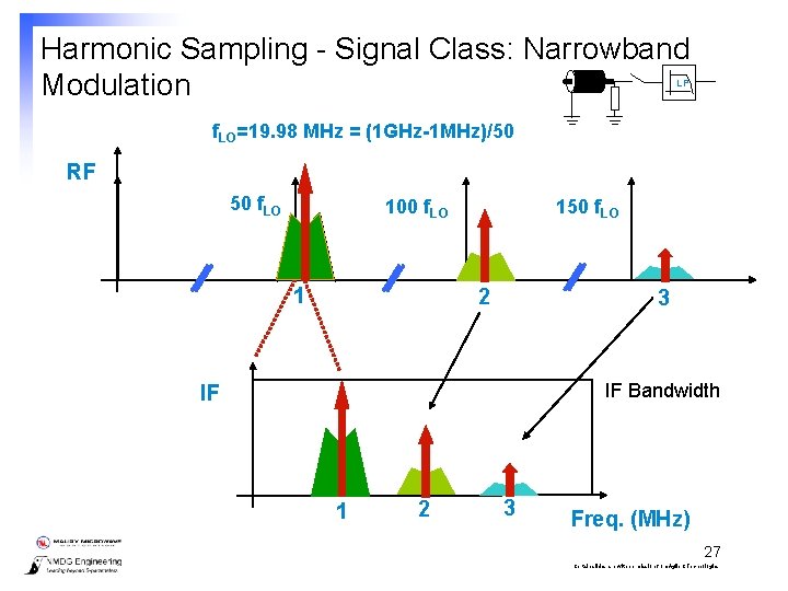
Harmonic Sampling - Signal Class: Narrowband Modulation LP f. LO=19. 98 MHz = (1 GHz-1 MHz)/50 RF 50 f. LO 100 f. LO 1 150 f. LO 2 3 IF Bandwidth IF 1 2 3 Freq. (MHz) 27 Certain slides are with permission from Agilent Technologies

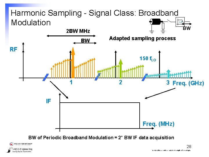
Harmonic Sampling - Signal Class: Broadband Modulation 2 BW MHz BW LP BW Adapted sampling process RF 150 f. LO 1 2 3 Freq. (GHz) IF Freq. (MHz) BW of Periodic Broadband Modulation = 2* BW IF data acquisition 28 Certain slides are with permission from Agilent Technologies

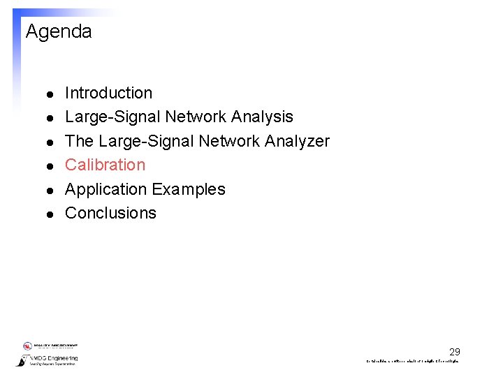
Agenda l l l Introduction Large-Signal Network Analysis The Large-Signal Network Analyzer Calibration Application Examples Conclusions 29 Certain slides are with permission from Agilent Technologies

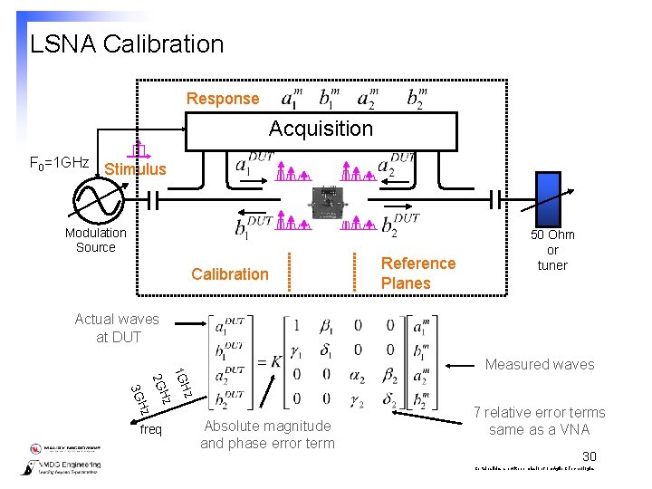
LSNA Calibration Response Acquisition F 0=1 GHz Stimulus Modulation Source Calibration Reference Planes 50 Ohm or tuner Actual waves at DUT 1 G Hz Hz Hz 2 G 3 G freq Measured waves Absolute magnitude and phase error term 7 relative error terms same as a VNA 30 Certain slides are with permission from Agilent Technologies

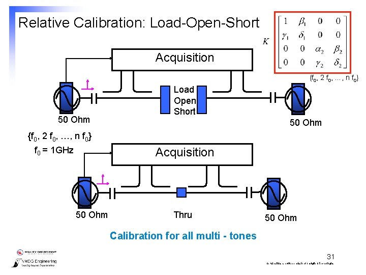
Relative Calibration: Load-Open-Short Acquisition {f 0, 2 f 0, …, n f 0} 50 Ohm Load Open Short 50 Ohm {f 0, 2 f 0, …, n f 0} f 0 = 1 GHz Acquisition 50 Ohm Thru 50 Ohm Calibration for all multi - tones 31 Certain slides are with permission from Agilent Technologies

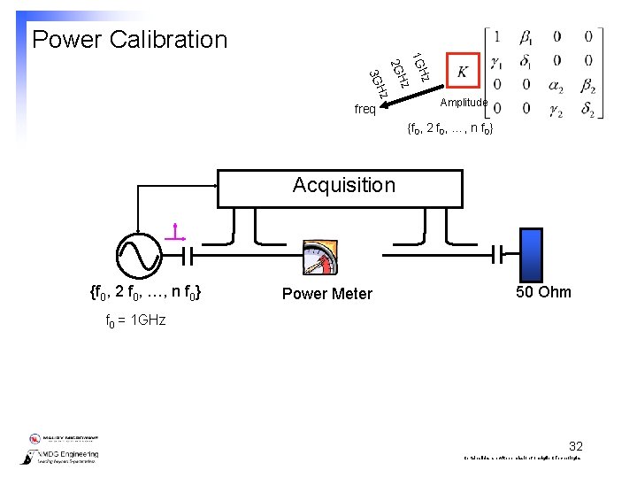
Power Calibration Hz 1 G Hz 2 G Hz 3 G freq Amplitude {f 0, 2 f 0, …, n f 0} Acquisition {f 0, 2 f 0, …, n f 0} Power Meter 50 Ohm f 0 = 1 GHz 32 Certain slides are with permission from Agilent Technologies

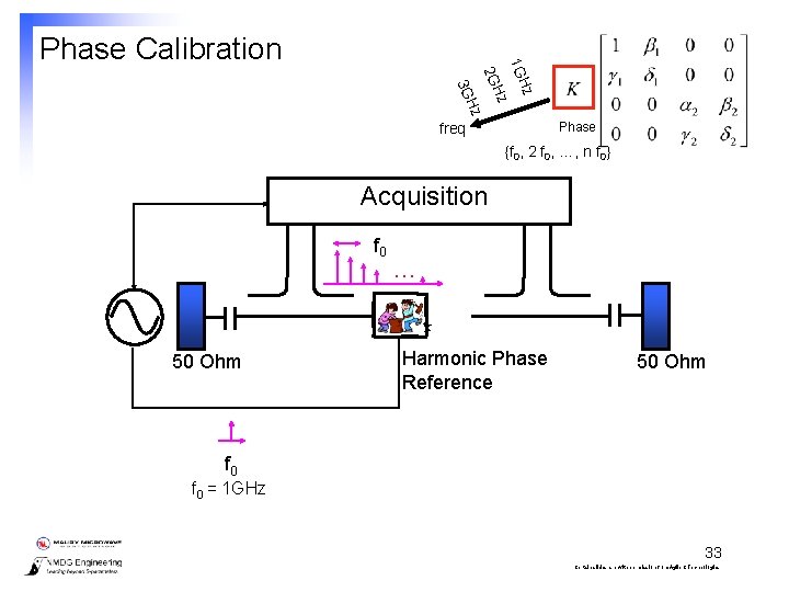
2 G Hz 3 G Hz 1 G Hz Phase Calibration Phase freq {f 0, 2 f 0, …, n f 0} Acquisition f 0 50 Ohm . . . Harmonic Phase Reference 50 Ohm f 0 = 1 GHz 33 Certain slides are with permission from Agilent Technologies

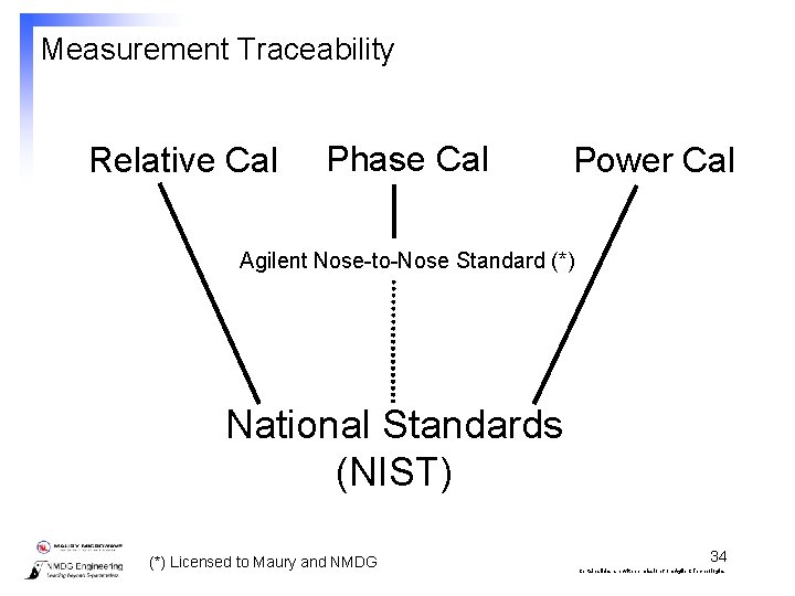
Measurement Traceability Relative Cal Phase Cal Power Cal Agilent Nose-to-Nose Standard (*) National Standards (NIST) (*) Licensed to Maury and NMDG 34 Certain slides are with permission from Agilent Technologies

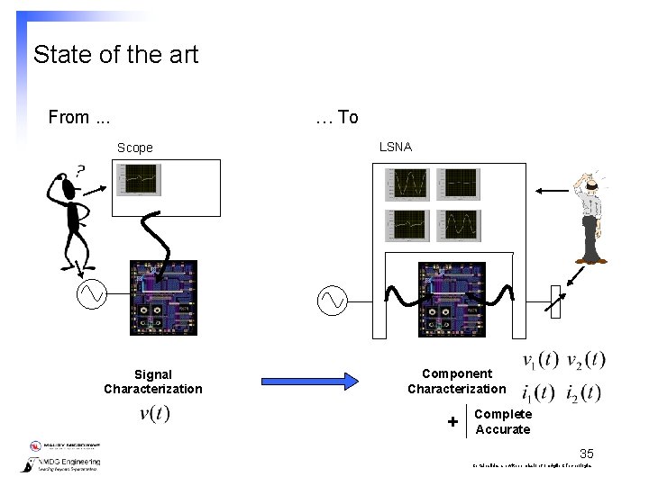
State of the art From. . . … To Scope Signal Characterization LSNA Component Characterization + Complete Accurate 35 Certain slides are with permission from Agilent Technologies

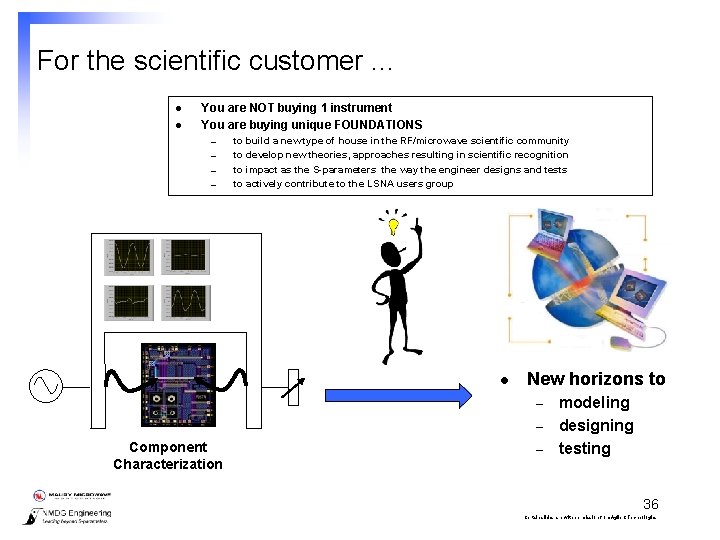
For the scientific customer. . . l l You are NOT buying 1 instrument You are buying unique FOUNDATIONS – – to build a new type of house in the RF/microwave scientific community to develop new theories, approaches resulting in scientific recognition to impact as the S-parameters the way the engineer designs and tests to actively contribute to the LSNA users group l New horizons to – – Component Characterization – modeling designing testing 36 Certain slides are with permission from Agilent Technologies

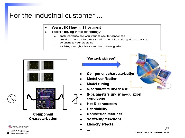
For the industrial customer. . . l l You are NOT buying 1 instrument You are buying into a technology – – – enabling you to see what your competitor cannot see creating a competitive advantage for you while working with us towards solutions to your problems evolving through software and hardware upgrades “We work with you” l l l l Component Characterization l l Component characterization Model verification Model tuning S-parameters under CW S-parameters under modulation conditions Hot S-parameters Hot stability Conversion matrices Scattering functions Memory effects. . . 37 Certain slides are with permission from Agilent Technologies

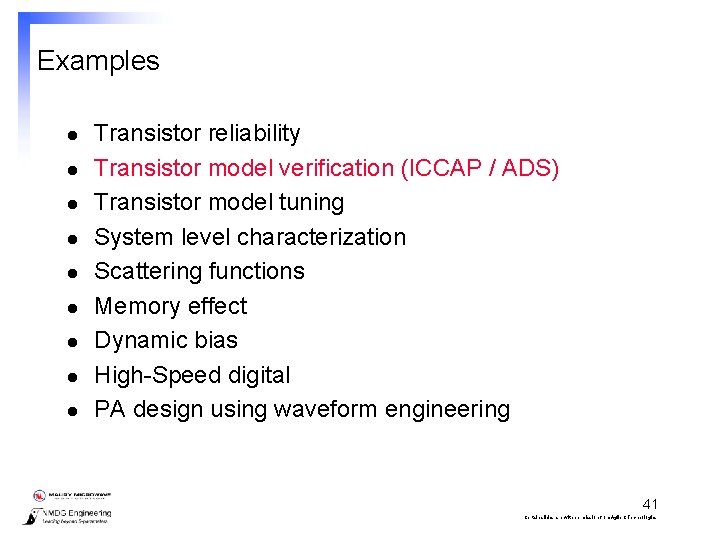
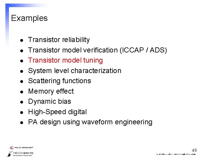
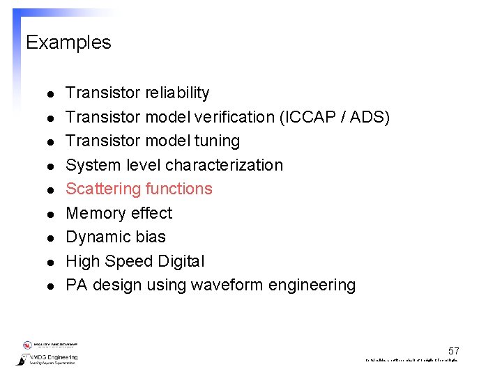
Examples l l l l l Transistor reliability Transistor model verification (ICCAP / ADS) Transistor model tuning System level characterization Scattering functions Memory effect Dynamic bias High-Speed digital PA design using waveform engineering 38 Certain slides are with permission from Agilent Technologies

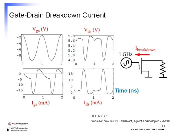
Gate-Drain Breakdown Current Time (ns) º TELEMIC / KUL º transistor provided by David Root, Agilent Technologies - MWTC 39 Certain slides are with permission from Agilent Technologies

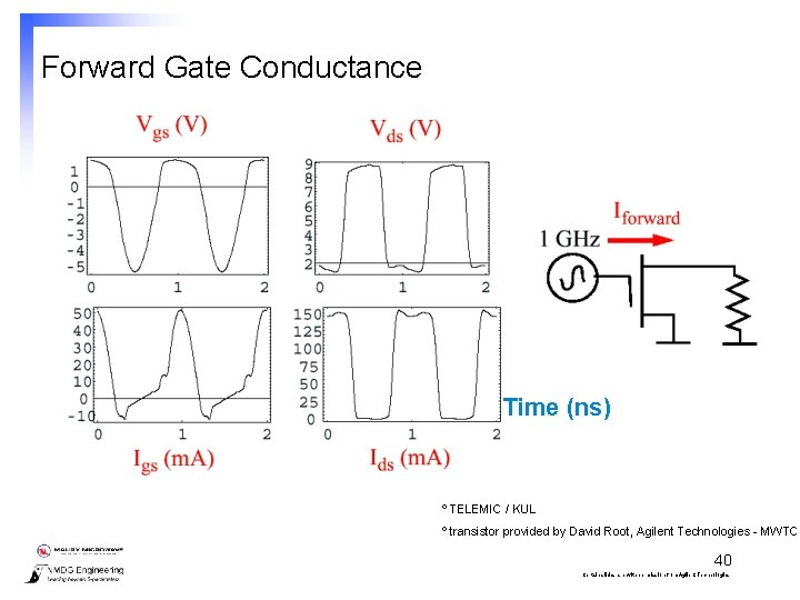
Forward Gate Conductance Time (ns) º TELEMIC / KUL º transistor provided by David Root, Agilent Technologies - MWTC 40 Certain slides are with permission from Agilent Technologies

Examples l l l l l Transistor reliability Transistor model verification (ICCAP / ADS) Transistor model tuning System level characterization Scattering functions Memory effect Dynamic bias High-Speed digital PA design using waveform engineering 41 Certain slides are with permission from Agilent Technologies

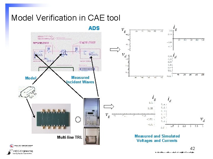
Model Verification in CAE tool ADS Model Measured Incident Waves Multi-line TRL Measured and Simulated Voltages and Currents 42 Certain slides are with permission from Agilent Technologies

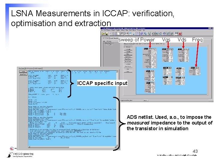
LSNA Measurements in ICCAP: verification, optimisation and extraction sweep of Power Vgs Vds Freq ICCAP specific input ADS netlist. Used, a. o. , to impose the measured impedance to the output of the transistor in simulation 43 Certain slides are with permission from Agilent Technologies

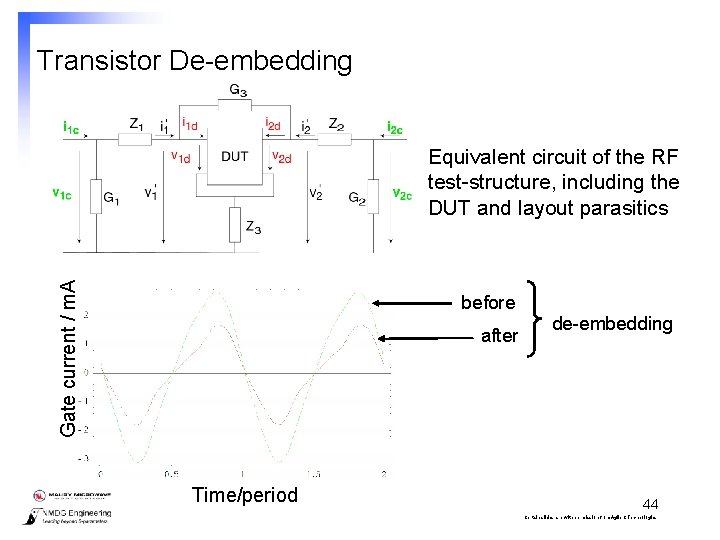
Transistor De-embedding Gate current / m. A Equivalent circuit of the RF test-structure, including the DUT and layout parasitics before after Time/period de-embedding 44 Certain slides are with permission from Agilent Technologies

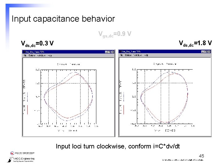
Input capacitance behavior Vgs, dc=0. 9 V Vds, dc=0. 3 V Vds, dc=1. 8 V Input loci turn clockwise, conform i=C*dv/dt 45 Certain slides are with permission from Agilent Technologies

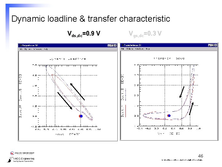
Dynamic loadline & transfer characteristic Vds, dc=0. 9 V Vgs, dc=0. 3 V 46 Certain slides are with permission from Agilent Technologies

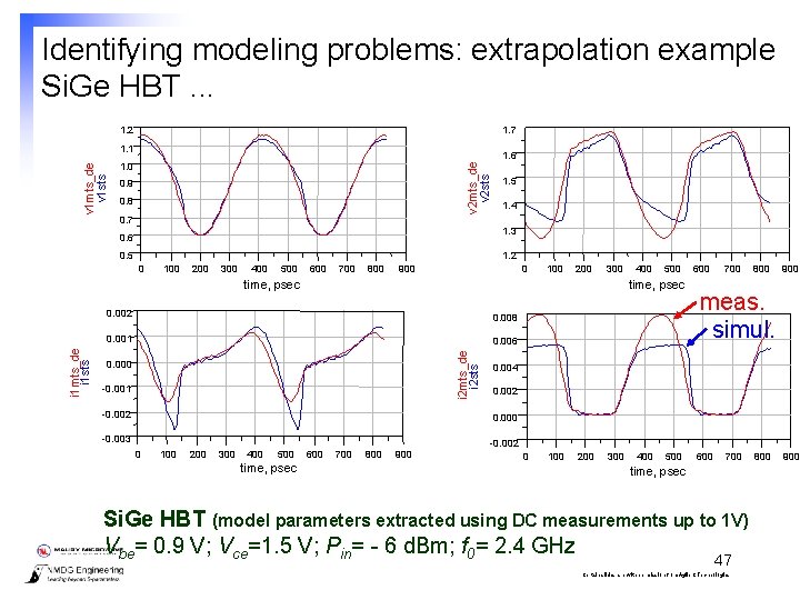
Identifying modeling problems: extrapolation example Si. Ge HBT. . . 1. 7 1. 2 1. 6 1. 0 v 2 mts_de v 2 sts v 1 mts_de v 1 sts 1. 1 0. 9 0. 8 0. 7 1. 5 1. 4 1. 3 0. 6 0. 5 1. 2 0 100 200 300 400 500 600 700 800 900 0 100 200 300 500 time, psec 0. 002 0. 008 0. 001 0. 006 i 2 mts_de i 2 sts i 1 mts_de i 1 sts time, psec 400 0. 000 -0. 001 -0. 002 600 700 800 900 meas. simul. 0. 004 0. 002 0. 000 -0. 003 -0. 002 0 100 200 300 400 500 time, psec 600 700 800 900 0 100 200 300 400 500 600 700 time, psec Si. Ge HBT (model parameters extracted using DC measurements up to 1 V) Vbe= 0. 9 V; Vce=1. 5 V; Pin= - 6 d. Bm; f 0= 2. 4 GHz 47 Certain slides are with permission from Agilent Technologies 800 900

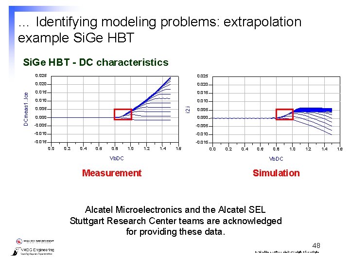
… Identifying modeling problems: extrapolation example Si. Ge HBT 0. 025 0. 020 0. 015 0. 010 0. 005 i 2. i DCmeas 1. . Ice Si. Ge HBT - DC characteristics 0. 005 0. 000 -0. 005 -0. 010 -0. 015 0. 0 0. 2 0. 4 0. 6 0. 8 1. 0 Vb. DC Measurement 1. 2 1. 4 1. 6 0. 0 0. 2 0. 4 0. 6 0. 8 1. 0 1. 2 1. 4 Vb. DC Simulation Alcatel Microelectronics and the Alcatel SEL Stuttgart Research Center teams are acknowledged for providing these data. 48 Certain slides are with permission from Agilent Technologies 1. 6

Examples l l l l l Transistor reliability Transistor model verification (ICCAP / ADS) Transistor model tuning System level characterization Scattering functions Memory effect Dynamic bias High-Speed digital PA design using waveform engineering 49 Certain slides are with permission from Agilent Technologies

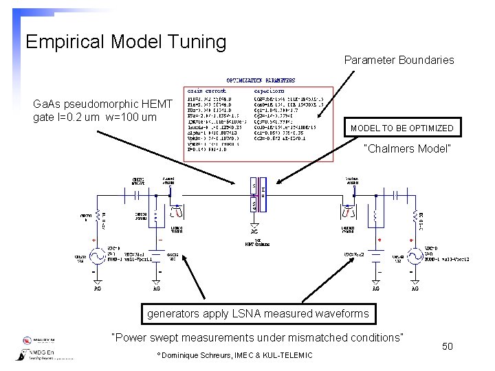
Empirical Model Tuning Parameter Boundaries Ga. As pseudomorphic HEMT gate l=0. 2 um w=100 um MODEL TO BE OPTIMIZED “Chalmers Model” generators apply LSNA measured waveforms “Power swept measurements under mismatched conditions” º Dominique Schreurs, IMEC & KUL-TELEMIC 50 Certain slides are with permission from Agilent Technologies

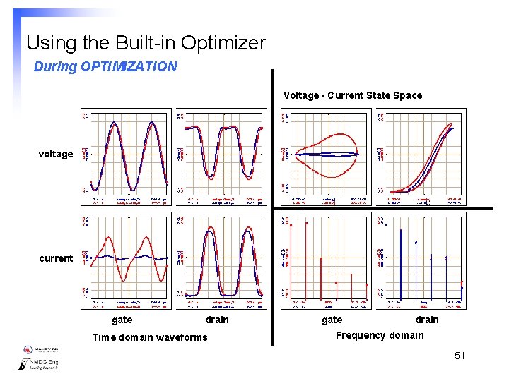
Using the Built-in Optimizer During OPTIMIZATION Voltage - Current State Space voltage current gate drain Time domain waveforms gate drain Frequency domain 51 Certain slides are with permission from Agilent Technologies

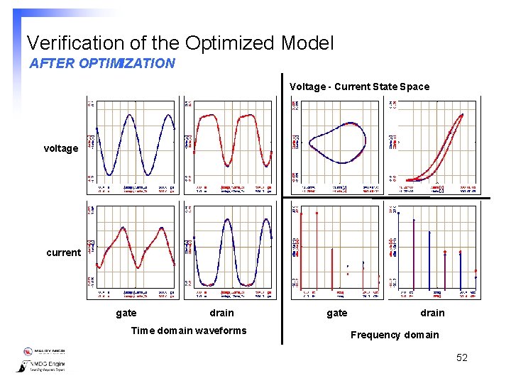
Verification of the Optimized Model AFTER OPTIMIZATION Voltage - Current State Space voltage current gate drain Time domain waveforms gate drain Frequency domain 52 Certain slides are with permission from Agilent Technologies

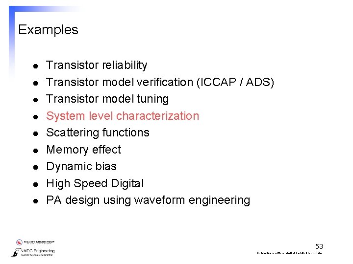
Examples l l l l l Transistor reliability Transistor model verification (ICCAP / ADS) Transistor model tuning System level characterization Scattering functions Memory effect Dynamic bias High Speed Digital PA design using waveform engineering 53 Certain slides are with permission from Agilent Technologies

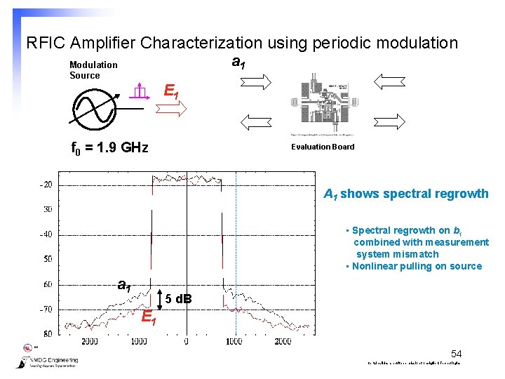
RFIC Amplifier Characterization using periodic modulation a 1 Modulation Source E 1 f 0 = 1. 9 GHz Evaluation Board A 1 shows spectral regrowth • Spectral regrowth on b 1 combined with measurement system mismatch • Nonlinear pulling on source a 1 5 d. B E 1 54 Certain slides are with permission from Agilent Technologies

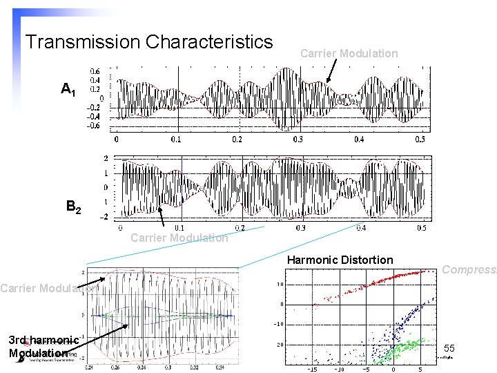
Transmission Characteristics Carrier Modulation A 1 B 2 Carrier Modulation Harmonic Distortion Compressi Carrier Modulation 3 rd harmonic Modulation 55 Certain slides are with permission from Agilent Technologies

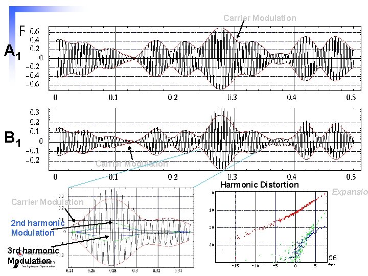
Carrier Modulation Reflection Characteristics A 1 B 1 Carrier Modulation Harmonic Distortion Expansion Carrier Modulation 2 nd harmonic Modulation 3 rd harmonic Modulation 56 Certain slides are with permission from Agilent Technologies

Examples l l l l l Transistor reliability Transistor model verification (ICCAP / ADS) Transistor model tuning System level characterization Scattering functions Memory effect Dynamic bias High Speed Digital PA design using waveform engineering 57 Certain slides are with permission from Agilent Technologies

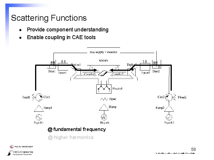
Scattering Functions l l Provide component understanding Enable coupling in CAE tools @ fundamental frequency @ higher harmonics 58 Certain slides are with permission from Agilent Technologies

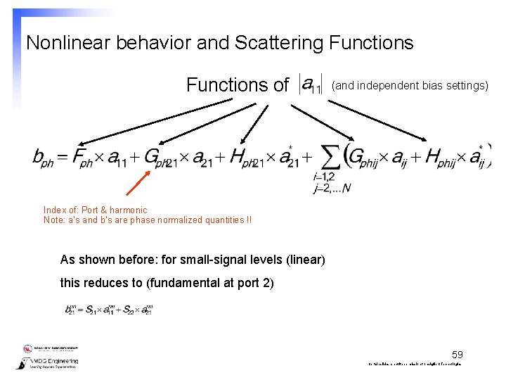
Nonlinear behavior and Scattering Functions of (and independent bias settings) Index of: Port & harmonic Note: a’s and b’s are phase normalized quantities !! As shown before: for small-signal levels (linear) this reduces to (fundamental at port 2) 59 Certain slides are with permission from Agilent Technologies

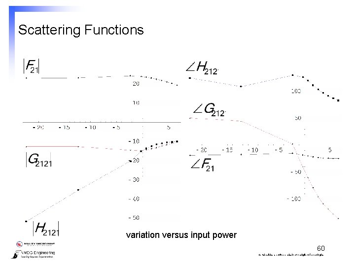
Scattering Functions variation versus input power 60 Certain slides are with permission from Agilent Technologies

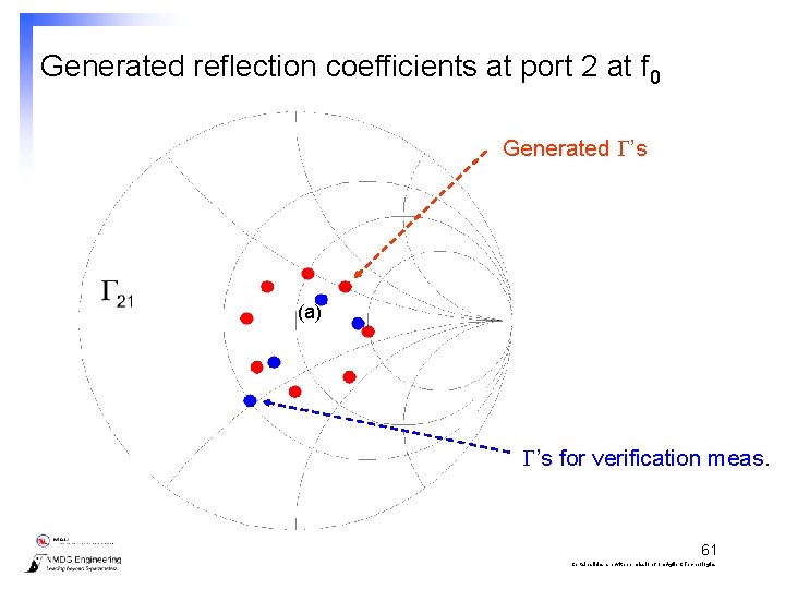
Generated reflection coefficients at port 2 at f 0 Generated ’s (a) ’s for verification meas. 61 Certain slides are with permission from Agilent Technologies

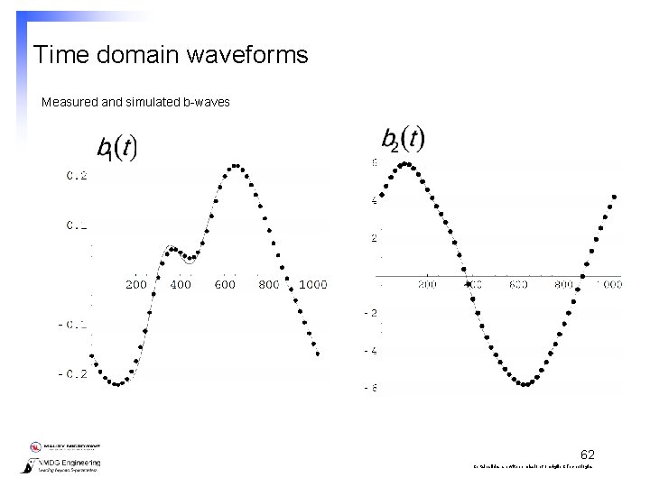
Time domain waveforms Measured and simulated b-waves 62 Certain slides are with permission from Agilent Technologies

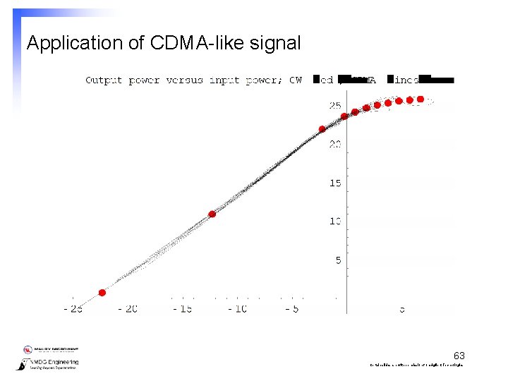
Application of CDMA-like signal 63 Certain slides are with permission from Agilent Technologies

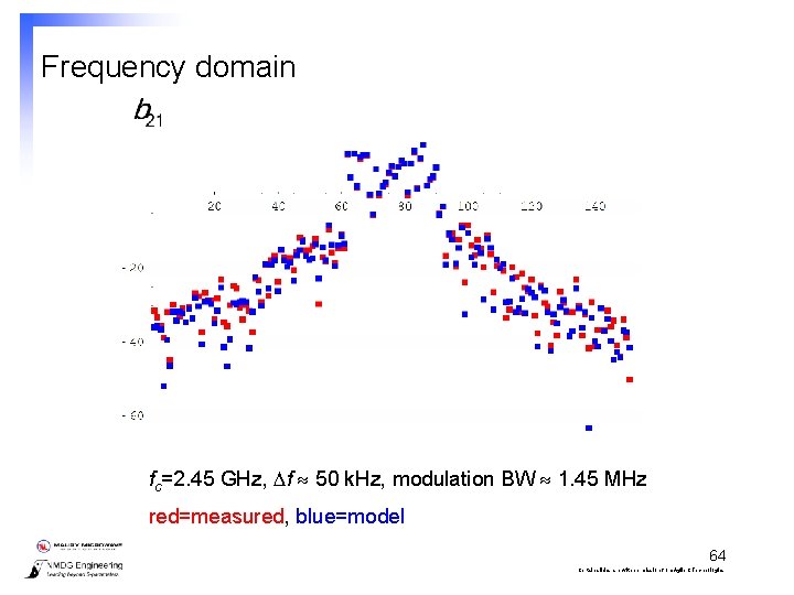
Frequency domain fc=2. 45 GHz, f 50 k. Hz, modulation BW 1. 45 MHz red=measured, blue=model 64 Certain slides are with permission from Agilent Technologies

Examples l l l l l Transistor reliability Transistor model verification (ICCAP / ADS) Transistor model tuning System level characterization Scattering functions Memory effect Dynamic bias High Speed Digital PA design using waveform engineering 65 Certain slides are with permission from Agilent Technologies

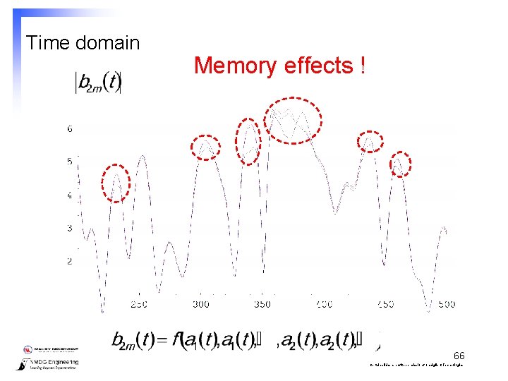
Time domain Memory effects ! 66 Certain slides are with permission from Agilent Technologies

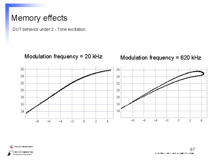
Memory effects DUT behavior under 2 - Tone excitation Modulation frequency = 20 k. Hz Modulation frequency = 620 k. Hz 67 Certain slides are with permission from Agilent Technologies

Examples l l l l l Transistor reliability Transistor model verification (ICCAP / ADS) Transistor model tuning System level characterization Scattering functions Memory effect Dynamic bias High Speed Digital PA design using waveform engineering 68 Certain slides are with permission from Agilent Technologies

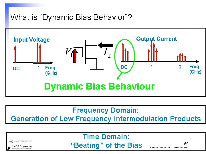
What is “Dynamic Bias Behavior”? Output Current Input Voltage DC 1 Freq. (GHz) 2 Dynamic Bias Behaviour Frequency Domain: Generation of Low Frequency Intermodulation Products Time Domain: “Beating” of the Bias 69 Certain slides are with permission from Agilent Technologies

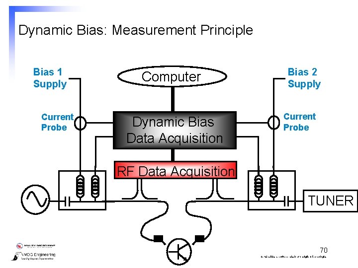
Dynamic Bias: Measurement Principle Bias 1 Supply Current Probe Computer Dynamic Bias Data Acquisition Bias 2 Supply Current Probe RF Data Acquisition TUNER 70 Certain slides are with permission from Agilent Technologies

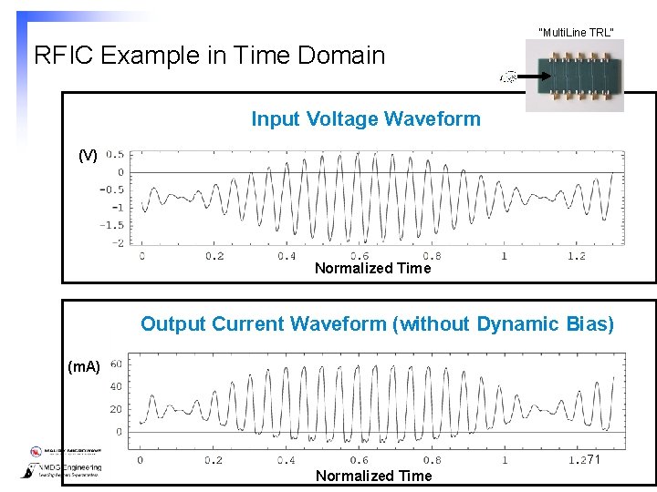
“Multi. Line TRL” RFIC Example in Time Domain Input Voltage Waveform (V) Normalized Time Output Current Waveform (without Dynamic Bias) (m. A) 71 Normalized Time Certain slides are with permission from Agilent Technologies

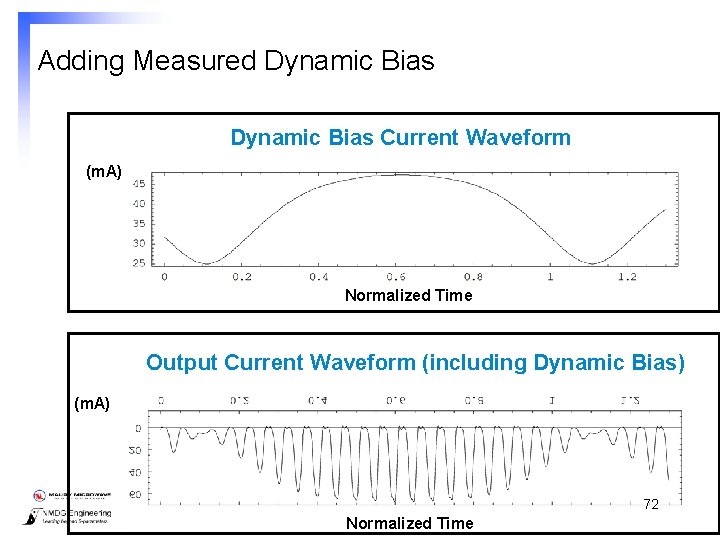
Adding Measured Dynamic Bias Current Waveform (m. A) Normalized Time Output Current Waveform (including Dynamic Bias) (m. A) 72 Normalized Time Certain slides are with permission from Agilent Technologies

Examples l l l l l Transistor reliability Transistor model verification (ICCAP / ADS) Transistor model tuning System level characterization Scattering functions Memory effect Dynamic bias High Speed Digital PA design using waveform engineering 73 Certain slides are with permission from Agilent Technologies

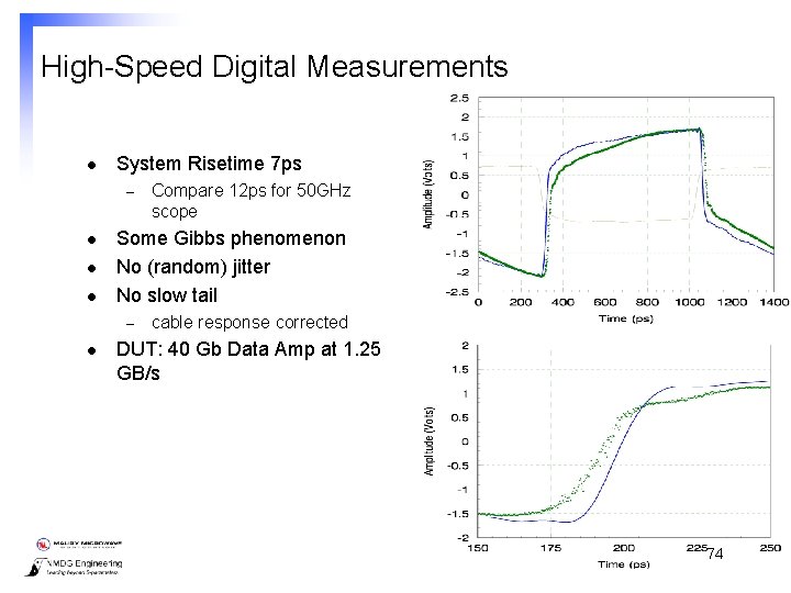
High-Speed Digital Measurements l System Risetime 7 ps – l l l Some Gibbs phenomenon No (random) jitter No slow tail – l Compare 12 ps for 50 GHz scope cable response corrected DUT: 40 Gb Data Amp at 1. 25 GB/s 74 Certain slides are with permission from Agilent Technologies

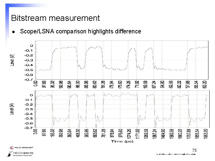
Bitstream measurement l Scope/LSNA comparison highlights difference 75 Certain slides are with permission from Agilent Technologies

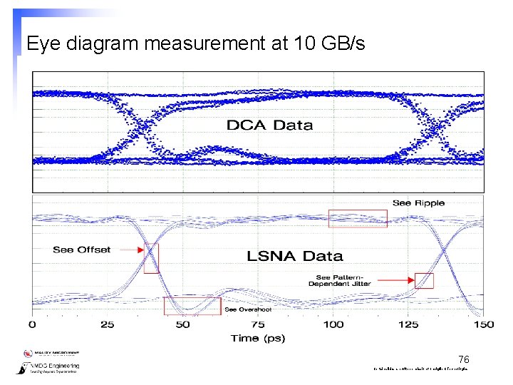
Eye diagram measurement at 10 GB/s 76 Certain slides are with permission from Agilent Technologies

Examples l l l l l Transistor reliability Transistor model verification (ICCAP / ADS) Transistor model tuning System level characterization Scattering functions Memory effect Dynamic bias High Speed Digital PA design using waveform engineering 77 Certain slides are with permission from Agilent Technologies

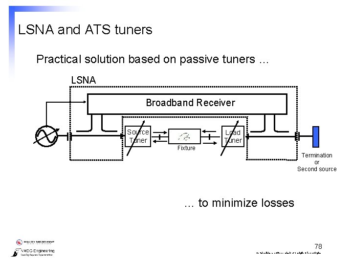
LSNA and ATS tuners Practical solution based on passive tuners … LSNA Broadband Receiver Source Tuner Load Tuner Fixture Termination or Second source … to minimize losses 78 Certain slides are with permission from Agilent Technologies

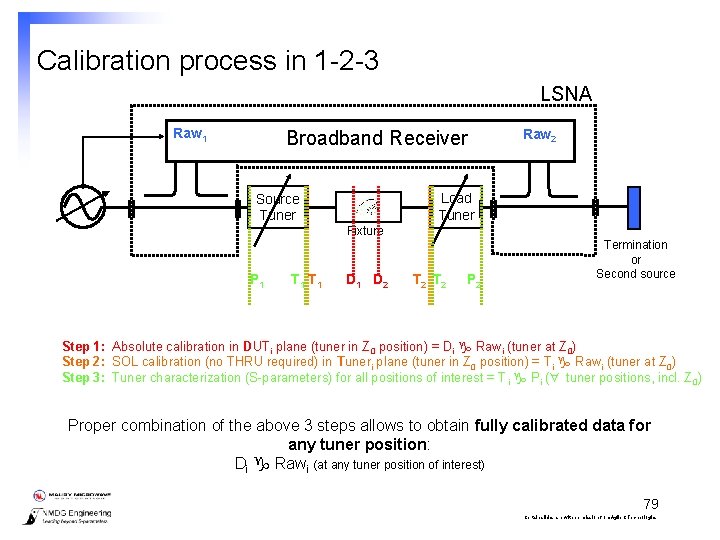
Calibration process in 1 -2 -3 LSNA Raw 1 Broadband Receiver Raw 2 Load Tuner Source Tuner Fixture P 1 T 1 D 2 T 2 P 2 Termination or Second source Step 1: Absolute calibration in DUTi plane (tuner in Z 0 position) = Di Rawi (tuner at Z 0) Step 2: SOL calibration (no THRU required) in Tuneri plane (tuner in Z 0 position) = Ti Rawi (tuner at Z 0) Step 3: Tuner characterization (S-parameters) for all positions of interest = T i Pi ( tuner positions, incl. Z 0) Proper combination of the above 3 steps allows to obtain fully calibrated data for any tuner position: Di Rawi (at any tuner position of interest) 79 Certain slides are with permission from Agilent Technologies

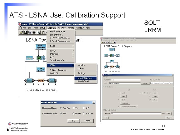
ATS - LSNA Use: Calibration Support SOLT LRRM 80 Certain slides are with permission from Agilent Technologies

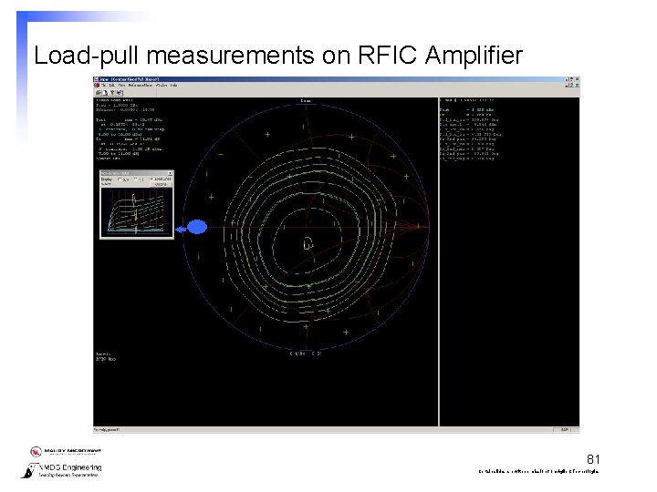
Load-pull measurements on RFIC Amplifier 81 Certain slides are with permission from Agilent Technologies

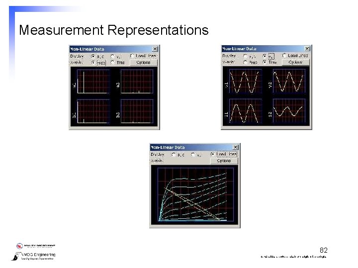
Measurement Representations 82 Certain slides are with permission from Agilent Technologies

Conclusions l Explanation of – – – Large-Signal Network Analysis concepts Block diagram, instrument and calibration process A limited set of examples l LSNA opens complete new horizons to improve the design and testing process in different ways when nonlinear behavior is envolved l Contact – – – Marc Vanden Bossche Marc. Vanden_Bossche@nmdg. be www. nmdg. be 83 Certain slides are with permission from Agilent Technologies