Laplacian Pyramids CS 194 Image Manipulation Computational Photography

Laplacian Pyramids CS 194: Image Manipulation & Computational Photography Many slides borrowed Alexei Efros, UC Berkeley, Fall 2017 from Steve Seitz

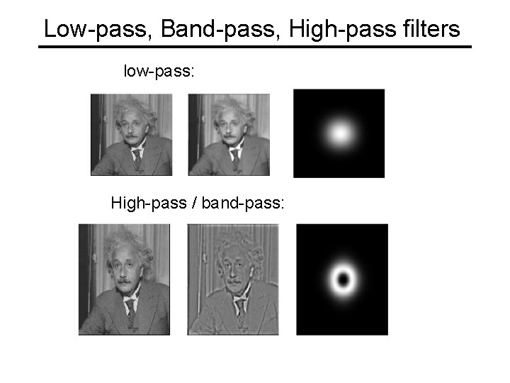
Low-pass, Band-pass, High-pass filters low-pass: High-pass / band-pass:

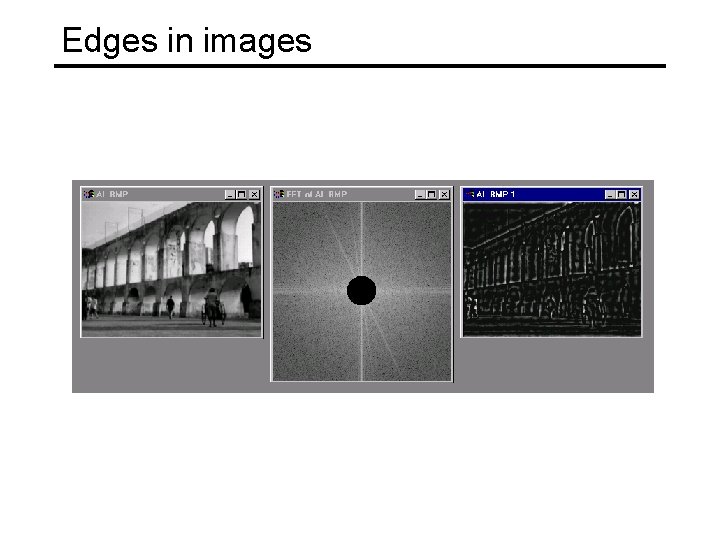
Edges in images

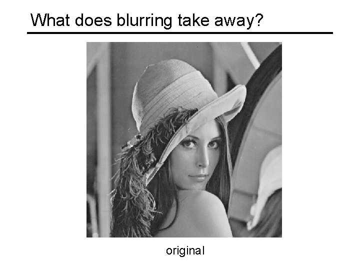
What does blurring take away? original

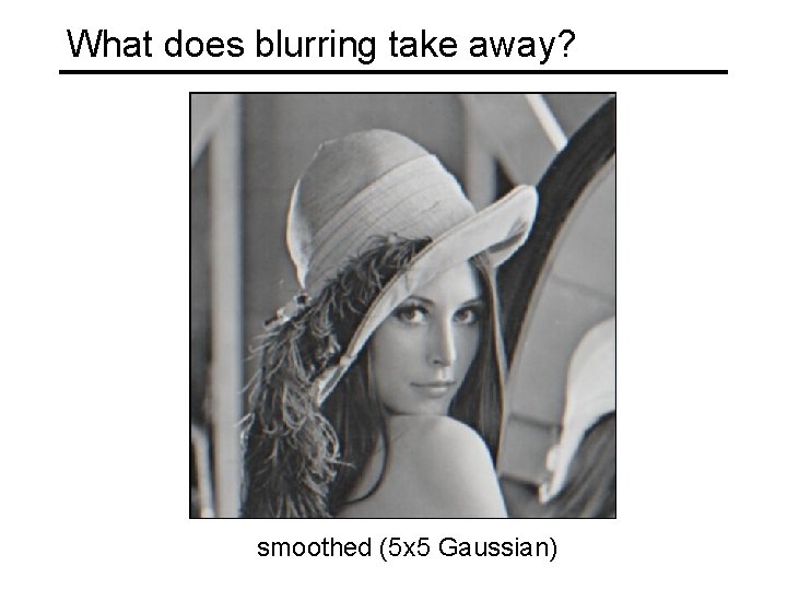
What does blurring take away? smoothed (5 x 5 Gaussian)

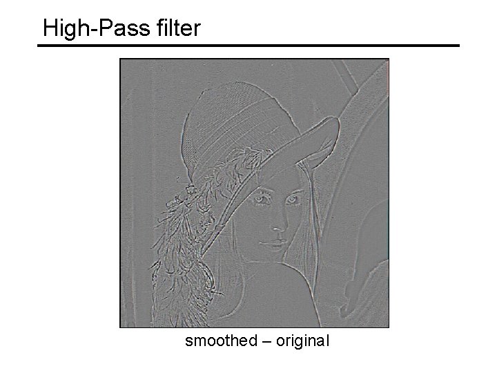
High-Pass filter smoothed – original

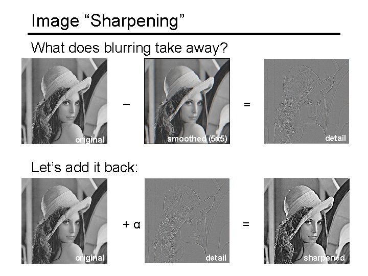
Image “Sharpening” What does blurring take away? – = detail smoothed (5 x 5) original Let’s add it back: +α original = detail sharpened

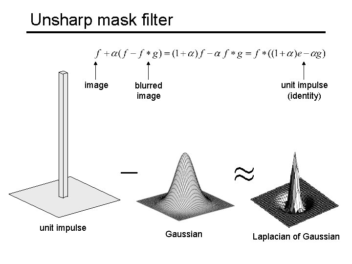
Unsharp mask filter image unit impulse (identity) blurred image Gaussian Laplacian of Gaussian

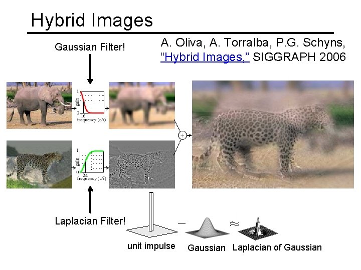
Hybrid Images Gaussian Filter! A. Oliva, A. Torralba, P. G. Schyns, “Hybrid Images, ” SIGGRAPH 2006 Laplacian Filter! unit impulse Gaussian Laplacian of Gaussian

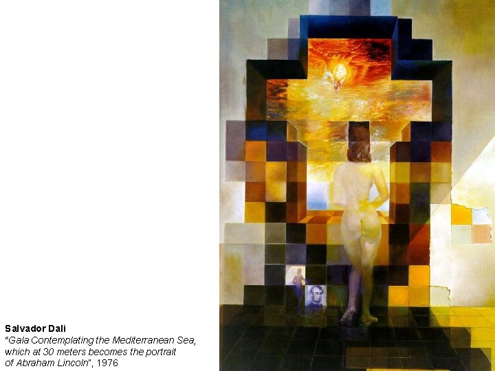
Salvador Dali “Gala Contemplating the Mediterranean Sea, which at 30 meters becomes the portrait of Abraham Lincoln”, 1976

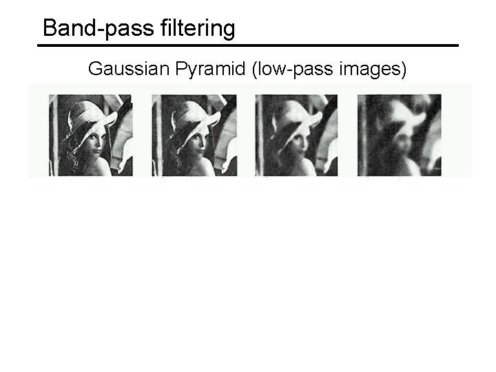
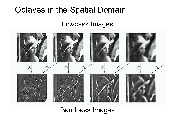
Band-pass filtering Gaussian Pyramid (low-pass images) Laplacian Pyramid (subband images) Created from Gaussian pyramid by subtraction

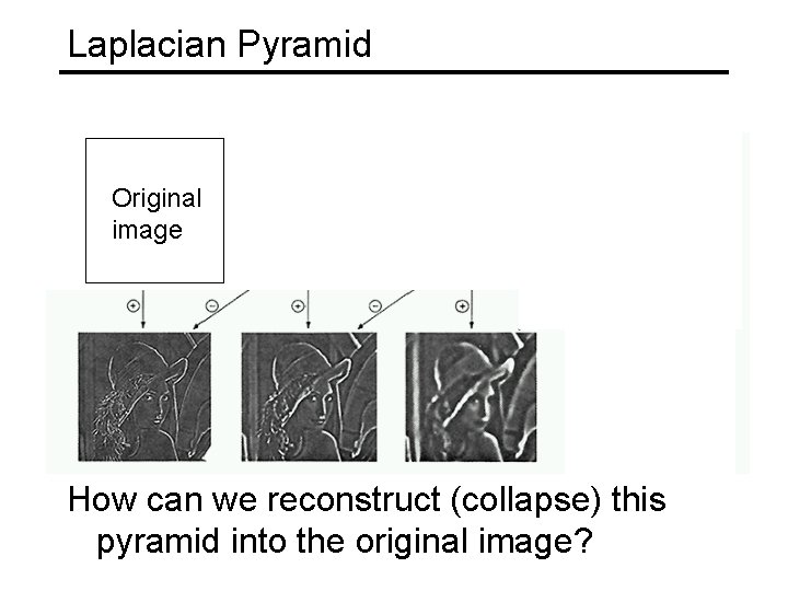
Laplacian Pyramid Need this! Original image How can we reconstruct (collapse) this pyramid into the original image?

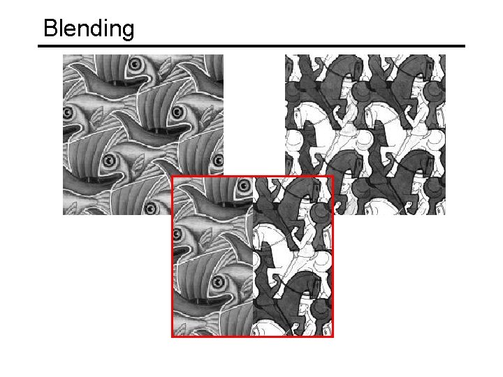
Blending

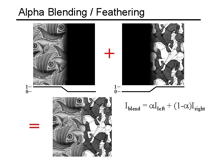
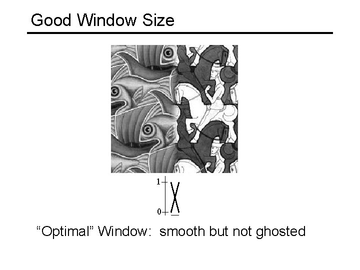
Alpha Blending / Feathering + 1 0 Iblend = a. Ileft + (1 -a)Iright =

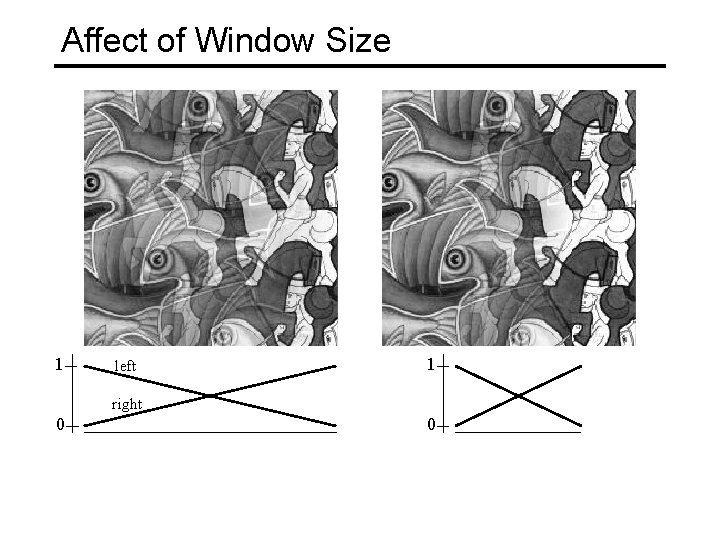
Affect of Window Size 1 left 1 right 0 0

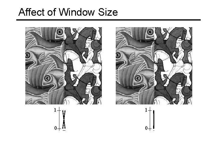
Affect of Window Size 1 1 0 0

Good Window Size 1 0 “Optimal” Window: smooth but not ghosted

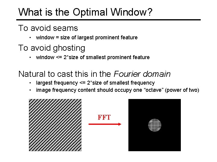
What is the Optimal Window? To avoid seams • window = size of largest prominent feature To avoid ghosting • window <= 2*size of smallest prominent feature Natural to cast this in the Fourier domain • largest frequency <= 2*size of smallest frequency • image frequency content should occupy one “octave” (power of two) FFT

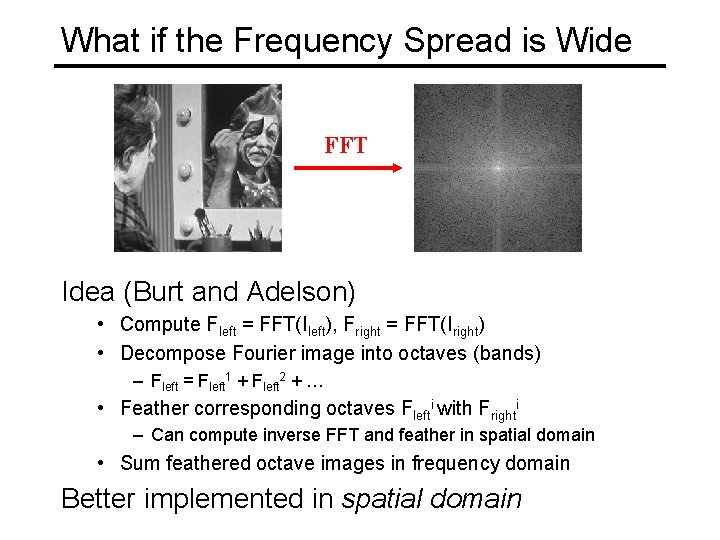
What if the Frequency Spread is Wide FFT Idea (Burt and Adelson) • Compute Fleft = FFT(Ileft), Fright = FFT(Iright) • Decompose Fourier image into octaves (bands) – Fleft = Fleft 1 + Fleft 2 + … • Feather corresponding octaves Flefti with Frighti – Can compute inverse FFT and feather in spatial domain • Sum feathered octave images in frequency domain Better implemented in spatial domain

Octaves in the Spatial Domain Lowpass Images Bandpass Images

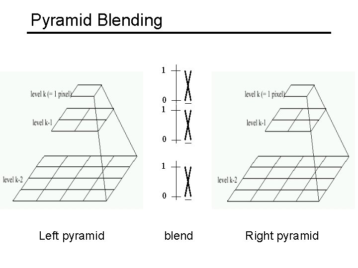
Pyramid Blending 1 0 1 0 Left pyramid blend Right pyramid

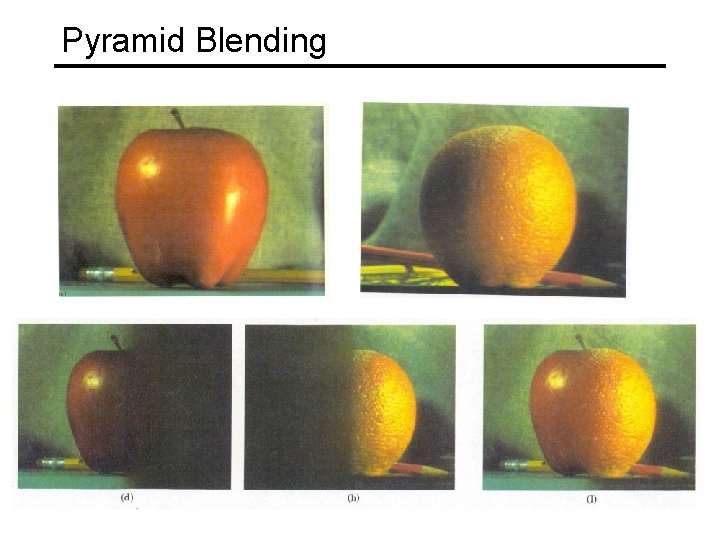
Pyramid Blending

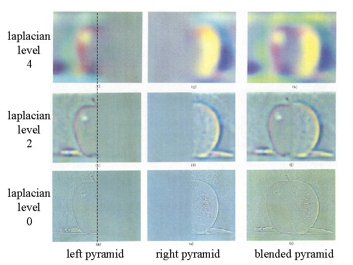
laplacian level 4 laplacian level 2 laplacian level 0 left pyramid right pyramid blended pyramid

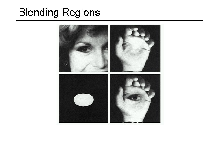
Blending Regions

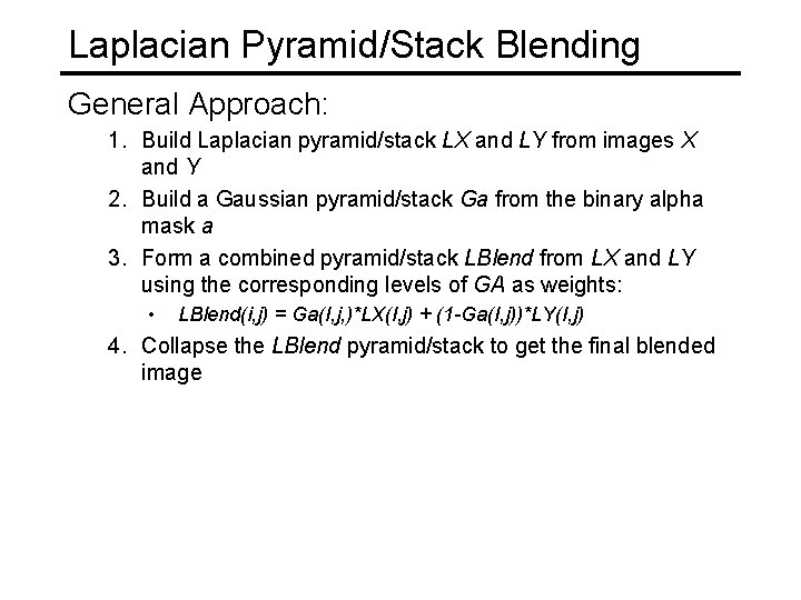
Laplacian Pyramid/Stack Blending General Approach: 1. Build Laplacian pyramid/stack LX and LY from images X and Y 2. Build a Gaussian pyramid/stack Ga from the binary alpha mask a 3. Form a combined pyramid/stack LBlend from LX and LY using the corresponding levels of GA as weights: • LBlend(i, j) = Ga(I, j, )*LX(I, j) + (1 -Ga(I, j))*LY(I, j) 4. Collapse the LBlend pyramid/stack to get the final blended image

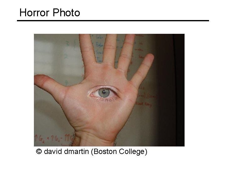
Horror Photo © david dmartin (Boston College)

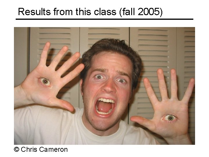
Results from this class (fall 2005) © Chris Cameron

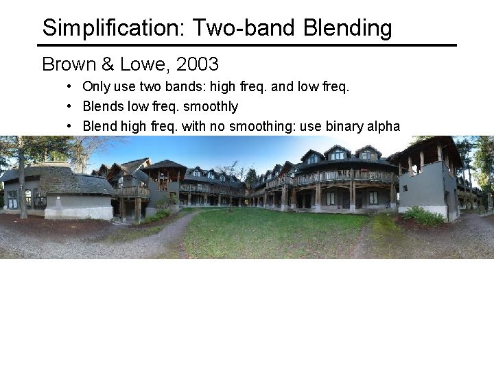
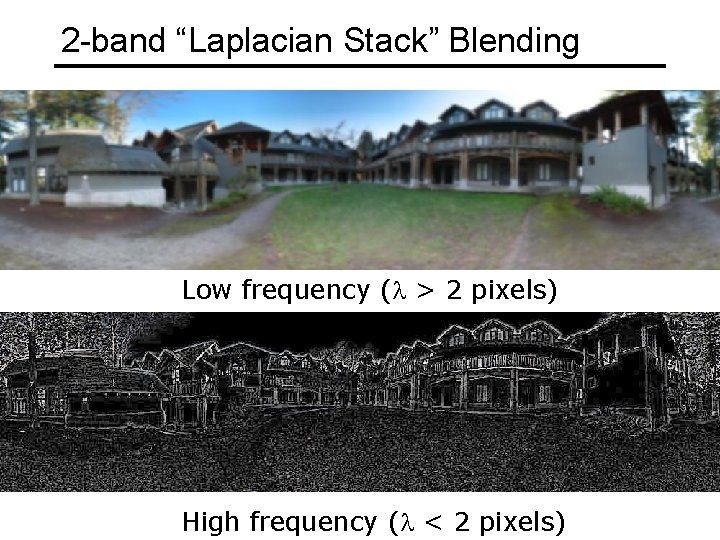
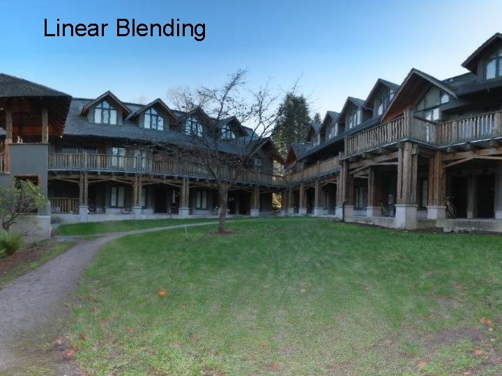
Simplification: Two-band Blending Brown & Lowe, 2003 • Only use two bands: high freq. and low freq. • Blends low freq. smoothly • Blend high freq. with no smoothing: use binary alpha

2 -band “Laplacian Stack” Blending Low frequency (l > 2 pixels) High frequency (l < 2 pixels)

Linear Blending

2 -band Blending

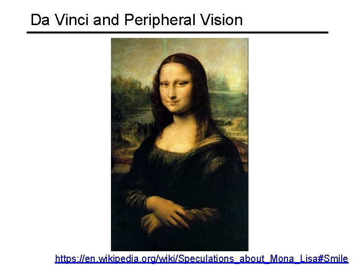
Da Vinci and Peripheral Vision https: //en. wikipedia. org/wiki/Speculations_about_Mona_Lisa#Smile

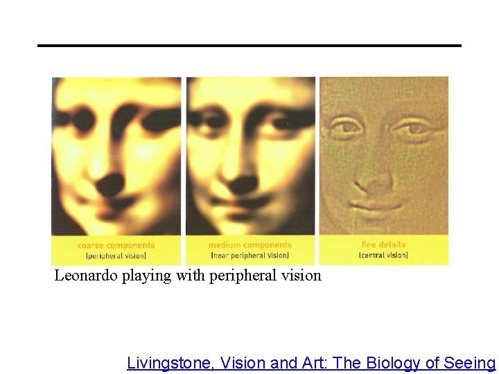
Leonardo playing with peripheral vision Livingstone, Vision and Art: The Biology of Seeing

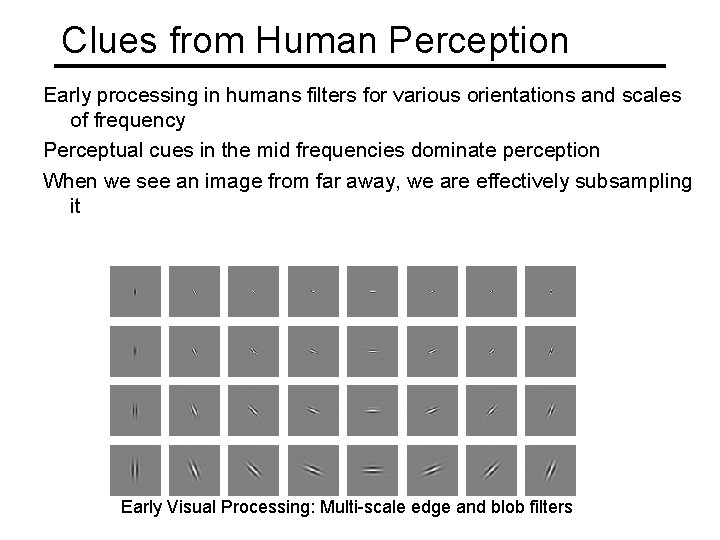
Clues from Human Perception Early processing in humans filters for various orientations and scales of frequency Perceptual cues in the mid frequencies dominate perception When we see an image from far away, we are effectively subsampling it Early Visual Processing: Multi-scale edge and blob filters

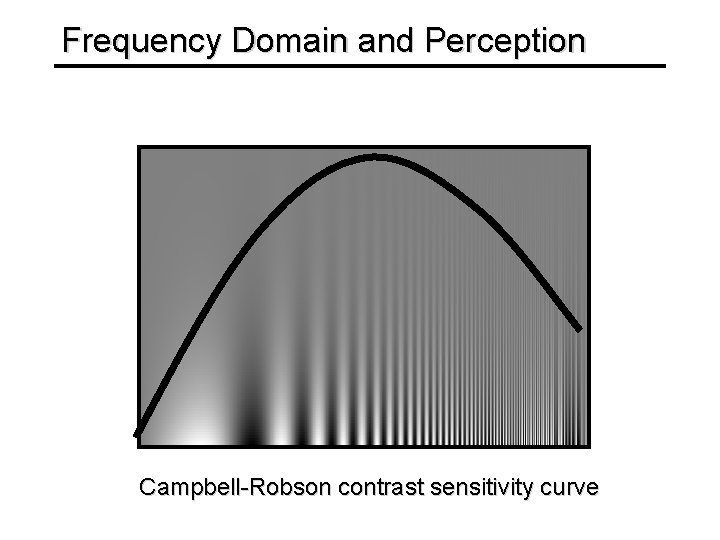
Frequency Domain and Perception Campbell-Robson contrast sensitivity curve

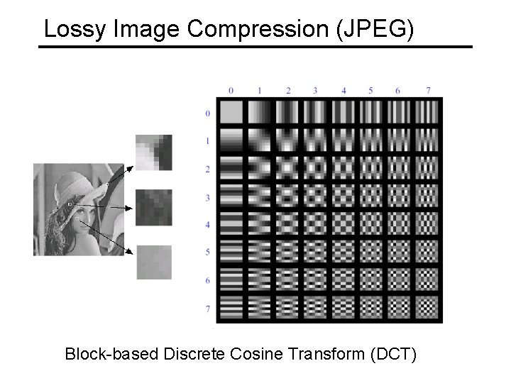
Lossy Image Compression (JPEG) Block-based Discrete Cosine Transform (DCT)

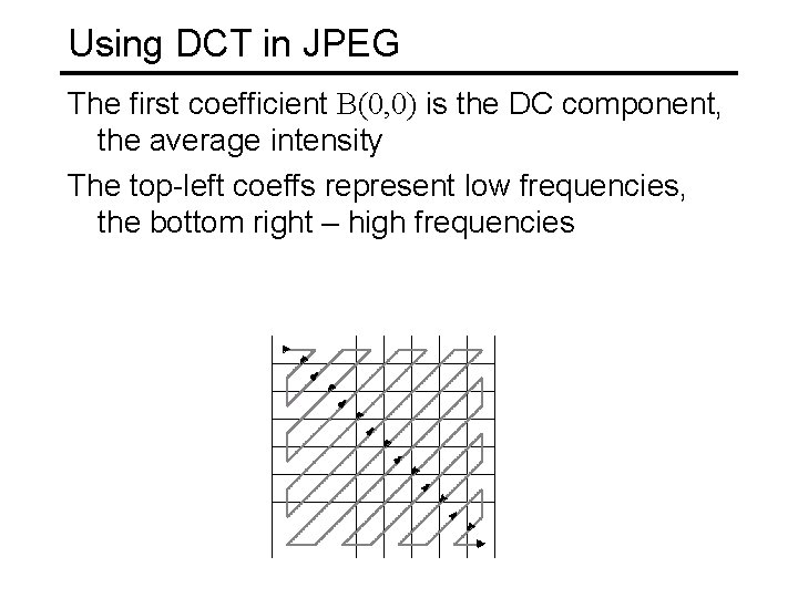
Using DCT in JPEG The first coefficient B(0, 0) is the DC component, the average intensity The top-left coeffs represent low frequencies, the bottom right – high frequencies

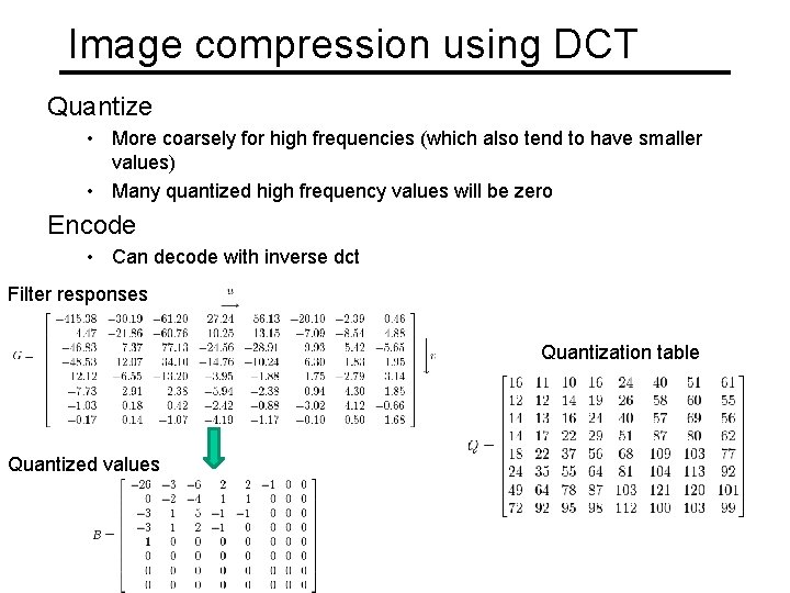
Image compression using DCT Quantize • More coarsely for high frequencies (which also tend to have smaller values) • Many quantized high frequency values will be zero Encode • Can decode with inverse dct Filter responses Quantization table Quantized values

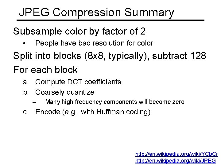
JPEG Compression Summary Subsample color by factor of 2 • People have bad resolution for color Split into blocks (8 x 8, typically), subtract 128 For each block a. Compute DCT coefficients b. Coarsely quantize – Many high frequency components will become zero c. Encode (e. g. , with Huffman coding) http: //en. wikipedia. org/wiki/YCb. Cr http: //en. wikipedia. org/wiki/JPEG

Block size in JPEG Block size • small block – faster – correlation exists between neighboring pixels • large block – better compression in smooth regions • It’s 8 x 8 in standard JPEG

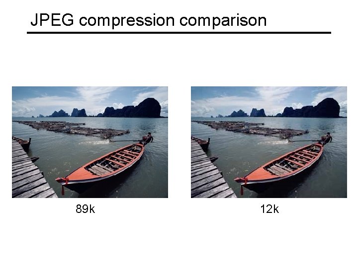
JPEG compression comparison 89 k 12 k