Laplaces Equation in 2 and 3 Dimensions Douglas

Laplace’s Equation in 2 and 3 Dimensions Douglas Wilhelm Harder, M. Math. LEL Department of Electrical and Computer Engineering University of Waterloo, Ontario, Canada ece. uwaterloo. ca dwharder@alumni. uwaterloo. ca © 2012 by Douglas Wilhelm Harder. Some rights reserved.

Laplace's Equation in 2 and 3 Dimensions Outline This topic discusses numerical solutions to the heatconduction/ diffusion equation: – – Discuss the physical problem and properties Examine the equation Consider boundary conditions in two and three dimensions Approximate the equation using a finite-difference equation • This will define a system of linear equations 2

Laplace's Equation in 2 and 3 Dimensions Outcomes Based Learning Objectives By the end of this laboratory, you will: – Understand Laplace’s equation – Understand how to approximate the equation in two and three dimensions using finite-difference equations – You will understand how the solutions may be approximated using a system of linear equations 3

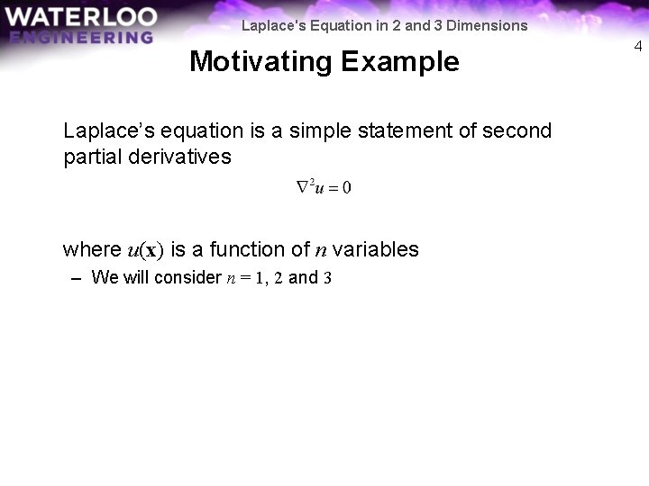
Laplace's Equation in 2 and 3 Dimensions Motivating Example Laplace’s equation is a simple statement of second partial derivatives where u(x) is a function of n variables – We will consider n = 1, 2 and 3 4

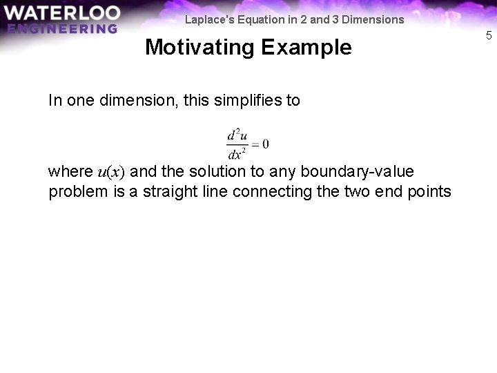
Laplace's Equation in 2 and 3 Dimensions Motivating Example In one dimension, this simplifies to where u(x) and the solution to any boundary-value problem is a straight line connecting the two end points 5

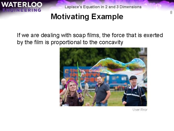
Laplace's Equation in 2 and 3 Dimensions Motivating Example If we are dealing with soap films, the force that exerted by the film is proportional to the concavity With concentrations, thermal energy and electric potentials, for a system to be in steady state, the forces exerted by the second derivatives with respect to concentration, thermal energy and electric potentials must be zero and cancel 6

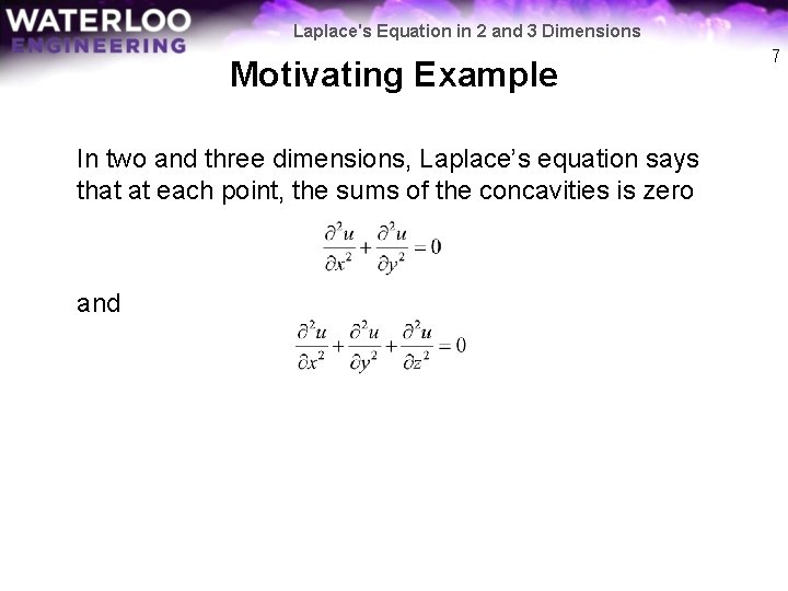
Laplace's Equation in 2 and 3 Dimensions Motivating Example In two and three dimensions, Laplace’s equation says that at each point, the sums of the concavities is zero and 7

Laplace's Equation in 2 and 3 Dimensions 8 Motivating Example If we are dealing with soap films, the force that is exerted by the film is proportional to the concavity User: Rror

Laplace's Equation in 2 and 3 Dimensions Motivating Example If we are dealing with a concentration, the concentration at any point will be the average of the concentrations around it – In the steady state, we do not expect one point to be more concentrated than everything around it 9

Laplace's Equation in 2 and 3 Dimensions Motivating Example If we are dealing with a thermal energy, thermal energy at any point will be the average of thermal energy around it – We do not expect, in the steady state, the temperature at one point to be higher or lower than all the points in the immediate neighbourhood 10

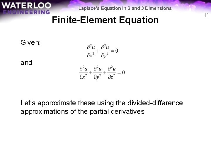
Laplace's Equation in 2 and 3 Dimensions Finite-Element Equation Given: and Let’s approximate these using the divided-difference approximations of the partial derivatives 11

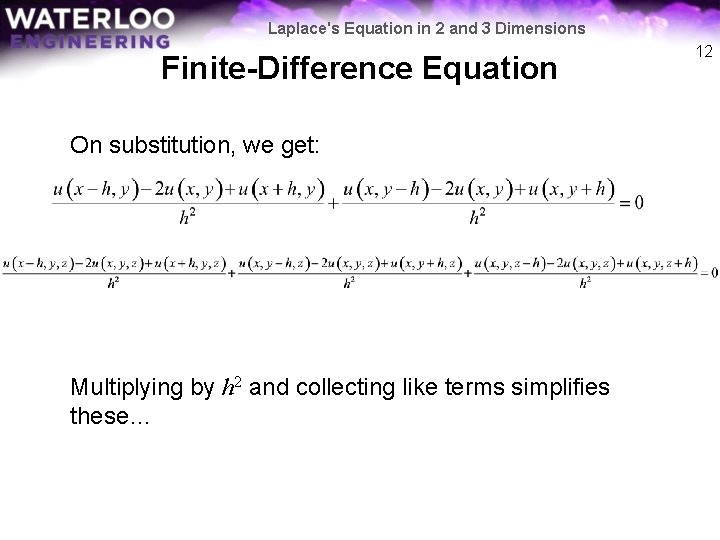
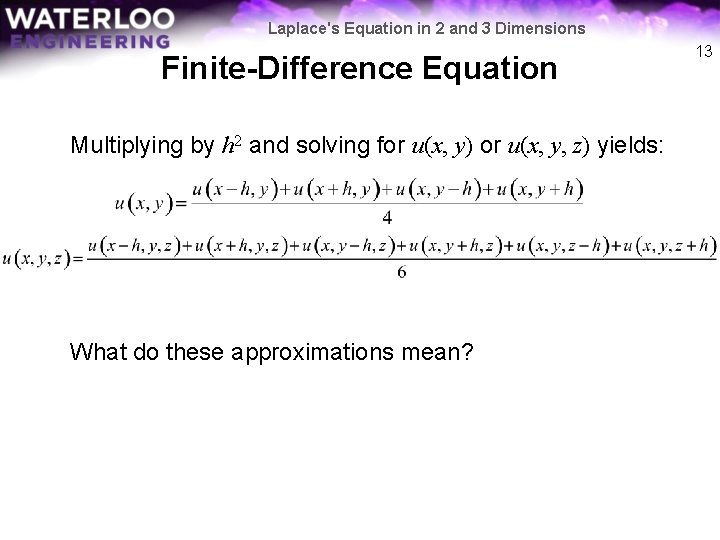
Laplace's Equation in 2 and 3 Dimensions Finite-Difference Equation On substitution, we get: Multiplying by h 2 and collecting like terms simplifies these… 12

Laplace's Equation in 2 and 3 Dimensions Finite-Difference Equation Multiplying by h 2 and solving for u(x, y) or u(x, y, z) yields: What do these approximations mean? 13

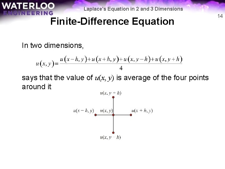
Laplace's Equation in 2 and 3 Dimensions Finite-Difference Equation In two dimensions, says that the value of u(x, y) is average of the four points around it 14

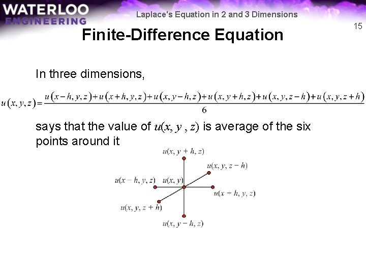
Laplace's Equation in 2 and 3 Dimensions Finite-Difference Equation In three dimensions, says that the value of u(x, y , z) is average of the six points around it 15

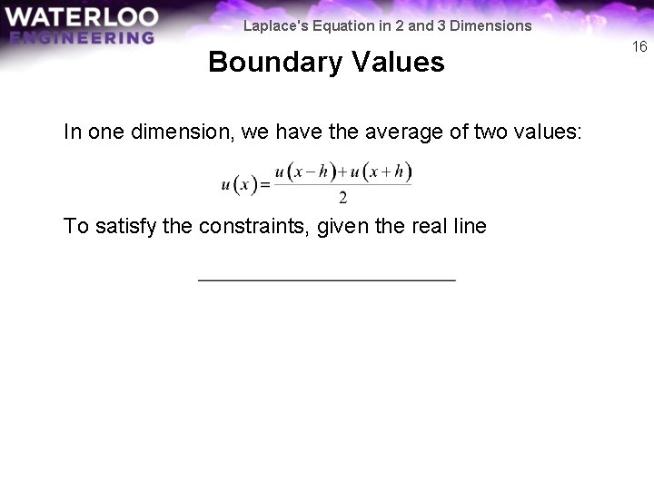
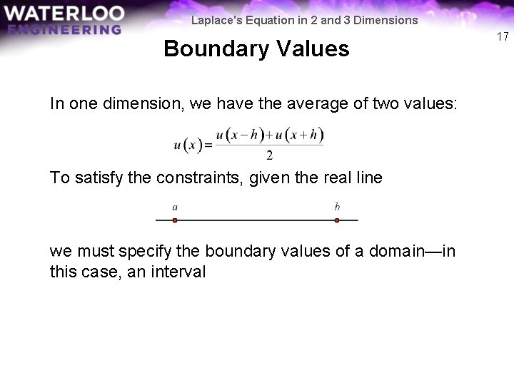
Laplace's Equation in 2 and 3 Dimensions Boundary Values In one dimension, we have the average of two values: To satisfy the constraints, given the real line 16

Laplace's Equation in 2 and 3 Dimensions Boundary Values In one dimension, we have the average of two values: To satisfy the constraints, given the real line we must specify the boundary values of a domain—in this case, an interval 17

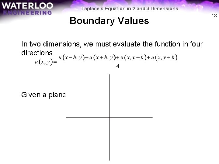
Laplace's Equation in 2 and 3 Dimensions Boundary Values In two dimensions, we must evaluate the function in four directions Given a plane, 18

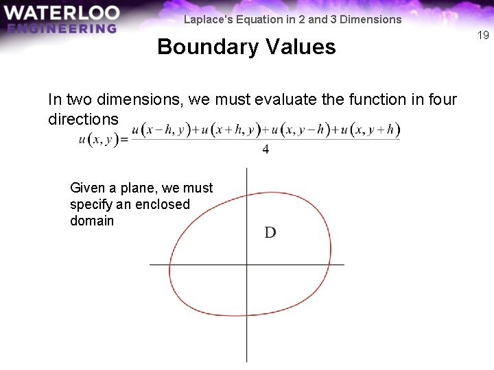
Laplace's Equation in 2 and 3 Dimensions Boundary Values In two dimensions, we must evaluate the function in four directions Given a plane, we must specify an enclosed domain 19

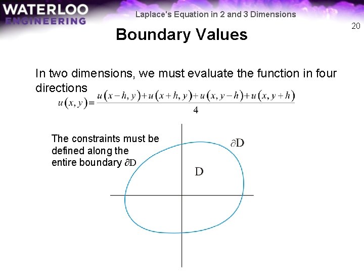
Laplace's Equation in 2 and 3 Dimensions Boundary Values In two dimensions, we must evaluate the function in four directions The constraints must be defined along the entire boundary ∂D 20

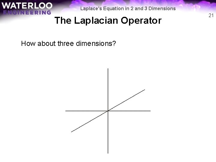
Laplace's Equation in 2 and 3 Dimensions The Laplacian Operator How about three dimensions? 21

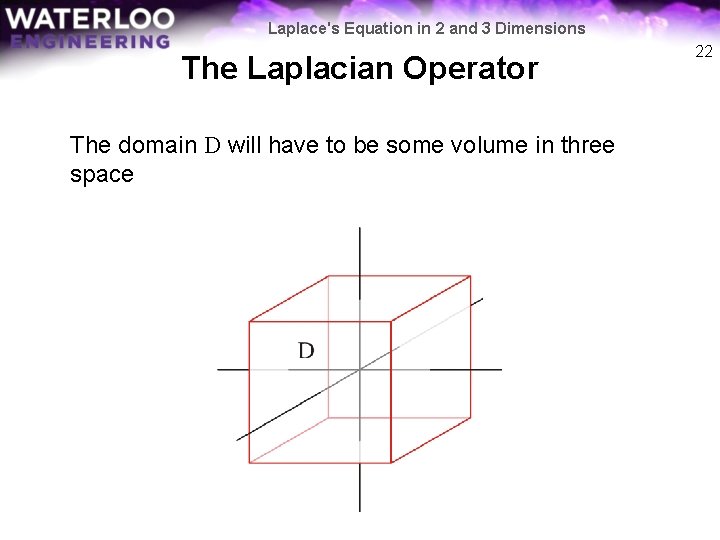
Laplace's Equation in 2 and 3 Dimensions The Laplacian Operator The domain D will have to be some volume in three space 22

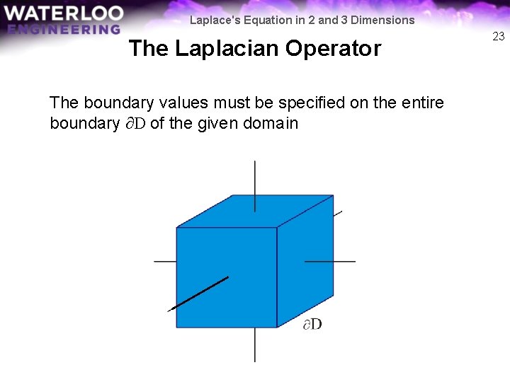
Laplace's Equation in 2 and 3 Dimensions The Laplacian Operator The boundary values must be specified on the entire boundary ∂D of the given domain 23

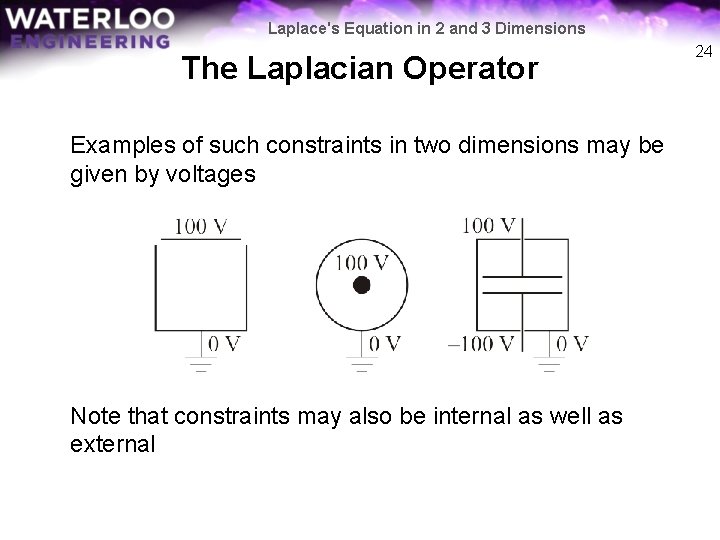
Laplace's Equation in 2 and 3 Dimensions The Laplacian Operator Examples of such constraints in two dimensions may be given by voltages Note that constraints may also be internal as well as external 24

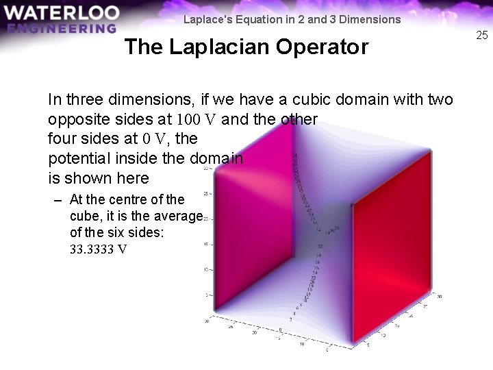
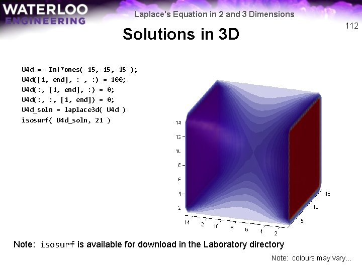
Laplace's Equation in 2 and 3 Dimensions The Laplacian Operator In three dimensions, if we have a cubic domain with two opposite sides at 100 V and the other four sides at 0 V, the potential inside the domain is shown here – At the centre of the cube, it is the average of the six sides: 33. 3333 V 25

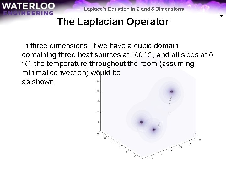
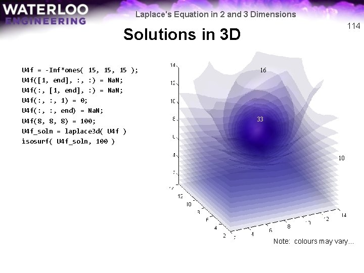
Laplace's Equation in 2 and 3 Dimensions The Laplacian Operator In three dimensions, if we have a cubic domain containing three heat sources at 100 °C, and all sides at 0 °C, the temperature throughout the room (assuming minimal convection) would be as shown 26

Laplace's Equation in 2 and 3 Dimensions The Laplacian Operator Given a closed wire frame, dipping the frame into a solution will produce a soap film – At each point, the concavities in the three directions will sum to zero This fails for soap bubbles because Laplace’s equation isn’t satisfied: there is an external force—the force of the air inside the bubble pushing out – It is a sphere because that is the shape that satisfies Poisson’s equation 27

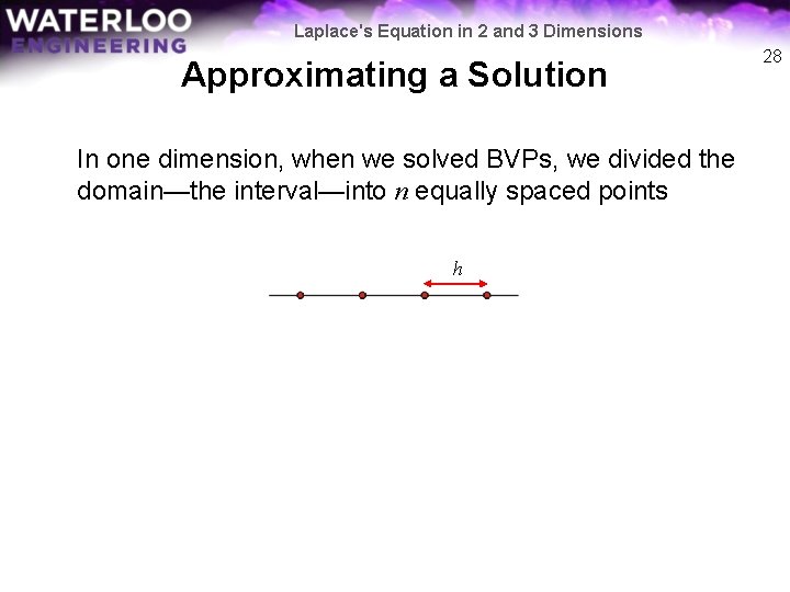
Laplace's Equation in 2 and 3 Dimensions Approximating a Solution In one dimension, when we solved BVPs, we divided the domain—the interval—into n equally spaced points h 28

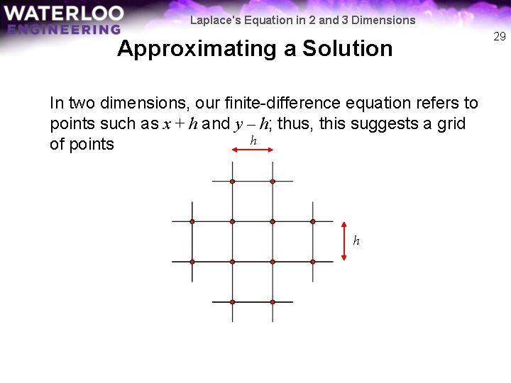
Laplace's Equation in 2 and 3 Dimensions Approximating a Solution In two dimensions, our finite-difference equation refers to points such as x + h and y – h; thus, this suggests a grid h of points h 29

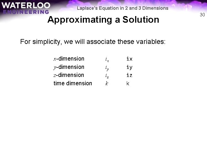
Laplace's Equation in 2 and 3 Dimensions Approximating a Solution For simplicity, we will associate these variables: x-dimension y-dimension z-dimension time dimension ix iy iz k 30

Laplace's Equation in 2 and 3 Dimensions Approximating a Solution Thus, if we had a rectangular domain in two dimensions – The boundary conditions would be defined on the edge of the rectangle 31

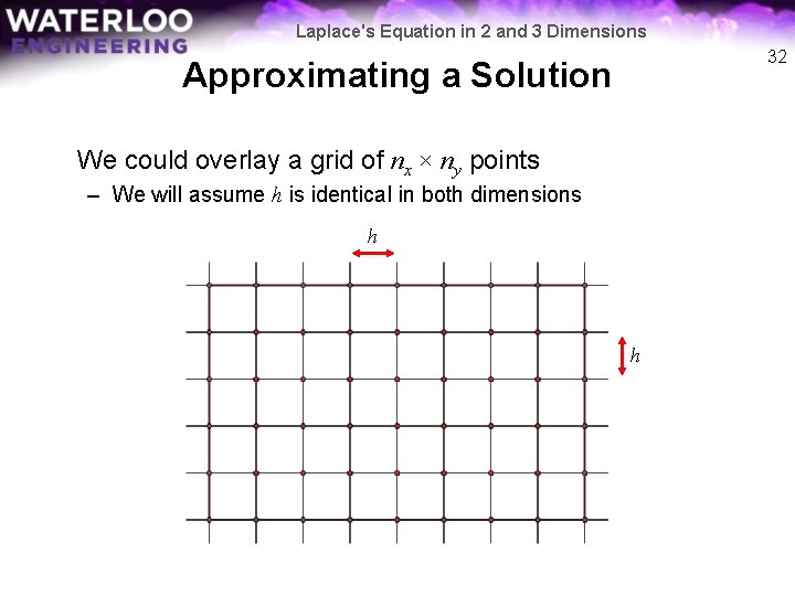
Laplace's Equation in 2 and 3 Dimensions 32 Approximating a Solution We could overlay a grid of nx × ny points – We will assume h is identical in both dimensions h h

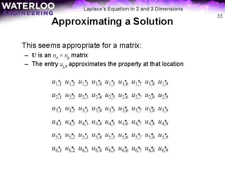
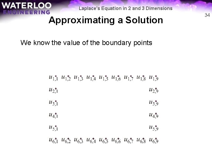
Laplace's Equation in 2 and 3 Dimensions Approximating a Solution This seems appropriate for a matrix: – U is an nx × ny matrix – The entry uj, k approximates the property at that location 33

Laplace's Equation in 2 and 3 Dimensions Approximating a Solution We know the value of the boundary points 34

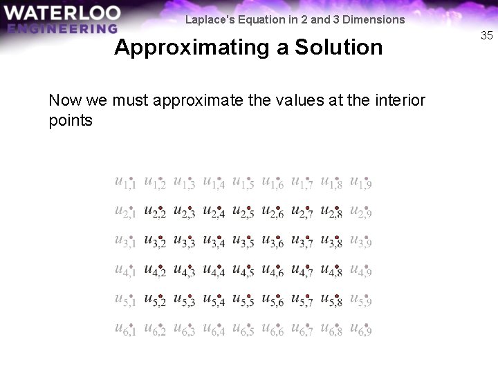
Laplace's Equation in 2 and 3 Dimensions Approximating a Solution Now we must approximate the values at the interior points 35

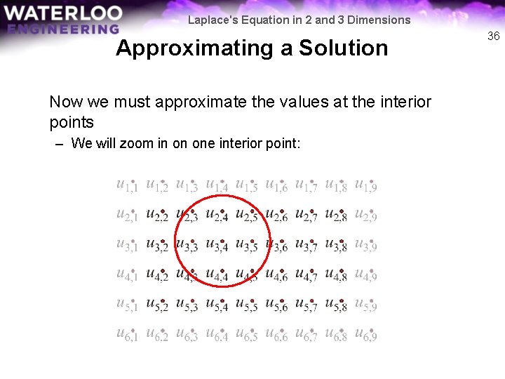
Laplace's Equation in 2 and 3 Dimensions Approximating a Solution Now we must approximate the values at the interior points – We will zoom in on one interior point: 36

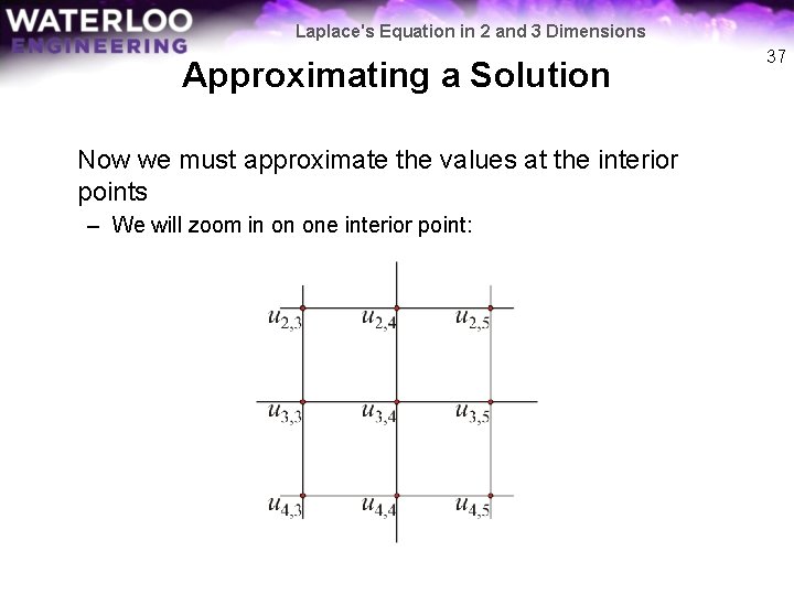
Laplace's Equation in 2 and 3 Dimensions Approximating a Solution Now we must approximate the values at the interior points – We will zoom in on one interior point: 37

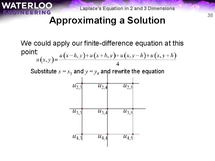
Laplace's Equation in 2 and 3 Dimensions Approximating a Solution We could apply our finite-difference equation at this point: Substitute x = x 3 and y = y 4 and rewrite the equation 38

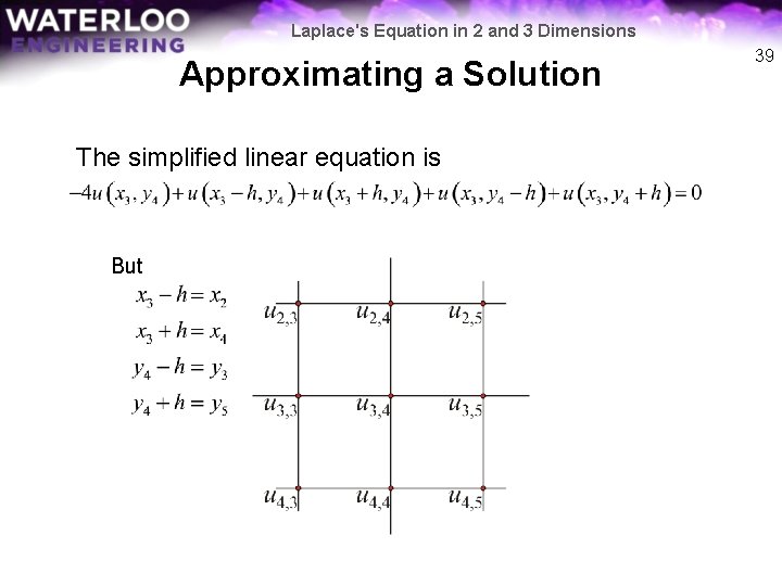
Laplace's Equation in 2 and 3 Dimensions Approximating a Solution The simplified linear equation is But 39

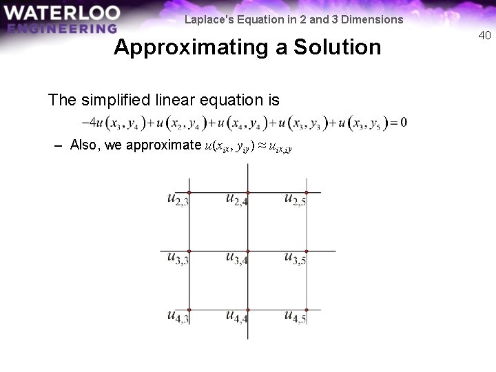
Laplace's Equation in 2 and 3 Dimensions Approximating a Solution The simplified linear equation is – Also, we approximate u(xix , yiy) ≈ uix , i y 40

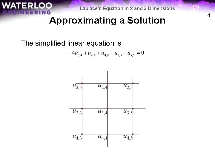
Laplace's Equation in 2 and 3 Dimensions Approximating a Solution The simplified linear equation is 41

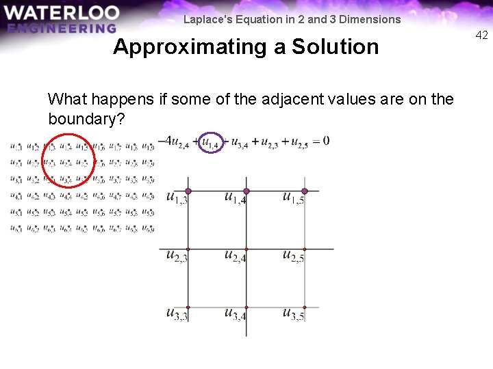
Laplace's Equation in 2 and 3 Dimensions Approximating a Solution What happens if some of the adjacent values are on the boundary? 42

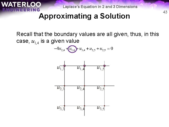
Laplace's Equation in 2 and 3 Dimensions Approximating a Solution Recall that the boundary values are all given, thus, in this case, u 1, 4 is a given value 43

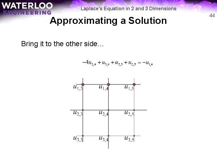
Laplace's Equation in 2 and 3 Dimensions Approximating a Solution Bring it to the other side… 44

Laplace's Equation in 2 and 3 Dimensions Approximating a Solution Thus, at each of the 28 interior points, we could write down a linear equation: 45

Laplace's Equation in 2 and 3 Dimensions Approximating a Solution Solve the system of equations, to get the approximate values at each of the interior points… 46

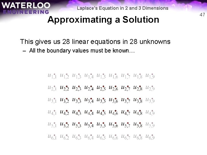
Laplace's Equation in 2 and 3 Dimensions Approximating a Solution This gives us 28 linear equations in 28 unknowns – All the boundary values must be known… 47

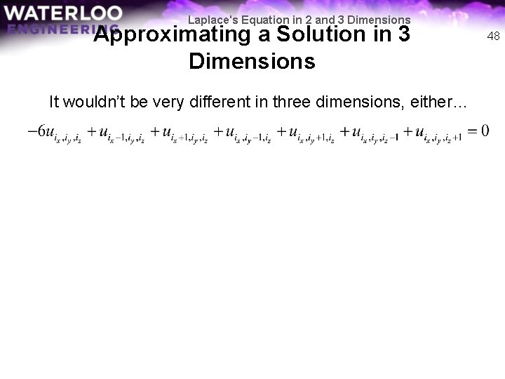
Laplace's Equation in 2 and 3 Dimensions Approximating a Solution in 3 Dimensions It wouldn’t be very different in three dimensions, either… 48

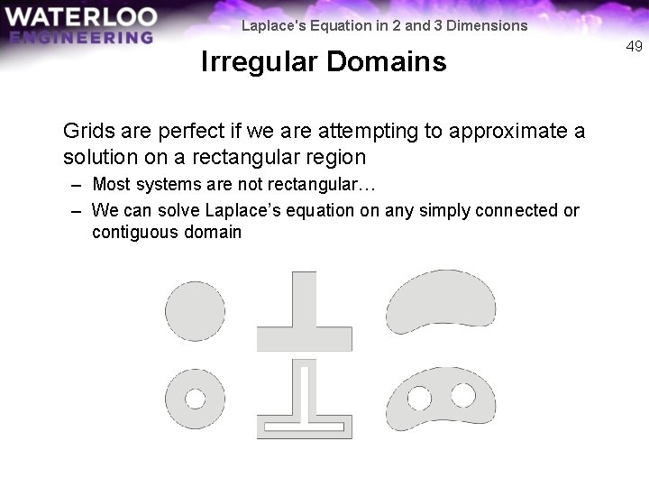
Laplace's Equation in 2 and 3 Dimensions Irregular Domains Grids are perfect if we are attempting to approximate a solution on a rectangular region – Most systems are not rectangular… – We can solve Laplace’s equation on any simply connected or contiguous domain 49

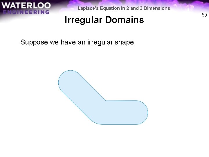
Laplace's Equation in 2 and 3 Dimensions Irregular Domains Suppose we have an irregular shape 50

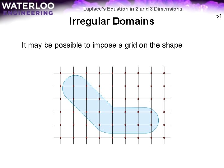
Laplace's Equation in 2 and 3 Dimensions Irregular Domains It may be possible to impose a grid on the shape 51

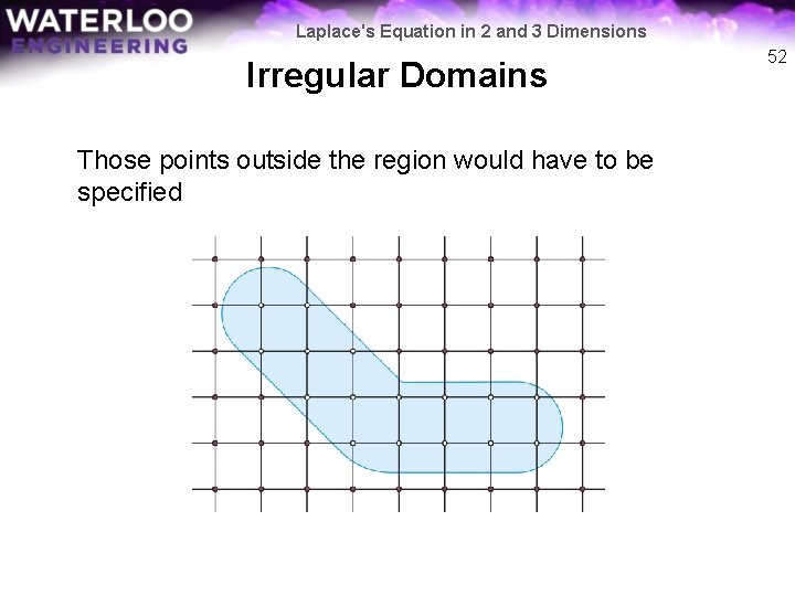
Laplace's Equation in 2 and 3 Dimensions Irregular Domains Those points outside the region would have to be specified 52

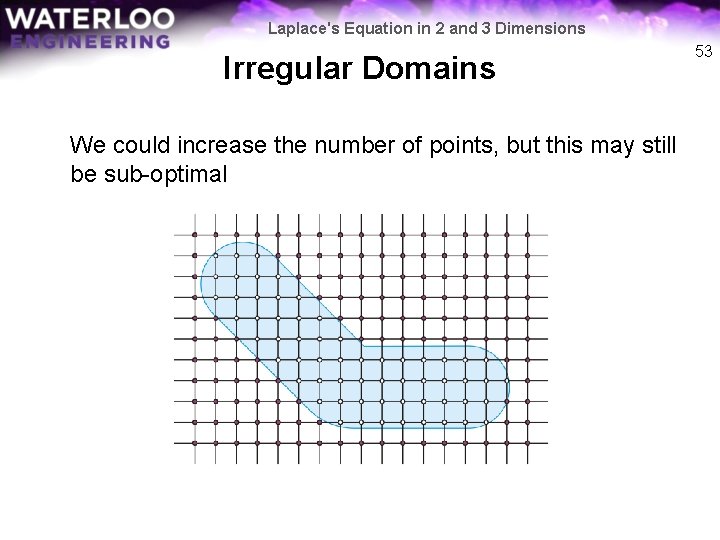
Laplace's Equation in 2 and 3 Dimensions Irregular Domains We could increase the number of points, but this may still be sub-optimal 53

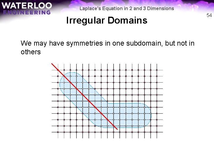
Laplace's Equation in 2 and 3 Dimensions Irregular Domains We may have symmetries in one subdomain, but not in others 54

Laplace's Equation in 2 and 3 Dimensions Finite Elements An alternative techniques, pioneered by Alexander Hrennikoff (a civil engineer) and Richard Courant in the early 1940 s – Finite elements allow the user to use tessellations – This divides the domain into triangular sub-domains in two dimensions or tetrahedral sub-domains in three dimensions The Nanotechnology students will see the finite-element method in their 3 B term 55

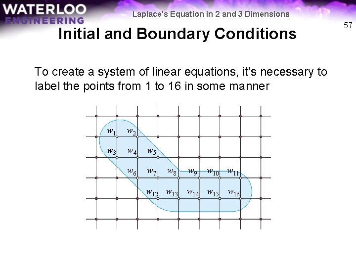
Laplace's Equation in 2 and 3 Dimensions Initial and Boundary Conditions When you consider this grid, there are 16 unknown points 56

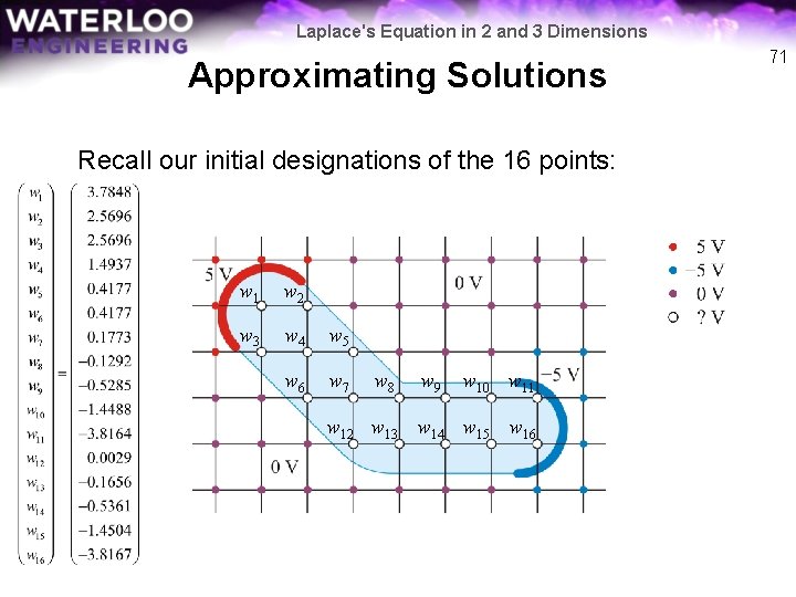
Laplace's Equation in 2 and 3 Dimensions Initial and Boundary Conditions To create a system of linear equations, it’s necessary to label the points from 1 to 16 in some manner w 1 w 2 w 3 w 4 w 5 w 6 w 7 w 8 w 9 w 10 w 11 w 12 w 13 w 14 w 15 w 16 57

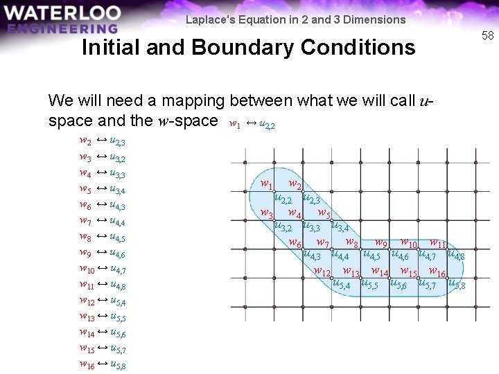
Laplace's Equation in 2 and 3 Dimensions Initial and Boundary Conditions We will need a mapping between what we will call uspace and the w-space w 1 ↔ u 2, 2 w 2 ↔ u 2, 3 w 3 ↔ u 3, 2 w 4 ↔ u 3, 3 w 5 ↔ u 3, 4 w 6 ↔ u 4, 3 w 7 ↔ u 4, 4 w 8 ↔ u 4, 5 w 9 ↔ u 4, 6 w 10 ↔ u 4, 7 w 11 ↔ u 4, 8 w 12 ↔ u 5, 4 w 13 ↔ u 5, 5 w 14 ↔ u 5, 6 w 15 ↔ u 5, 7 w 16 ↔ u 5, 8 w 1 w 2 u 2, 3 w 4 w 5 u 3, 2 u 3, 3 u 3, 4 w 6 w 7 w 8 w 9 w 10 w 11 u 4, 3 u 4, 4 u 4, 5 u 4, 6 u 4, 7 u 4, 8 w 12 w 13 w 14 w 15 w 16 u 5, 4 u 5, 5 u 5, 6 u 5, 7 u 5, 8 58

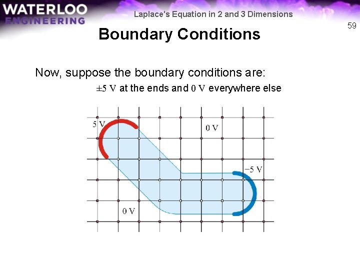
Laplace's Equation in 2 and 3 Dimensions Boundary Conditions Now, suppose the boundary conditions are: ± 5 V at the ends and 0 V everywhere else 59

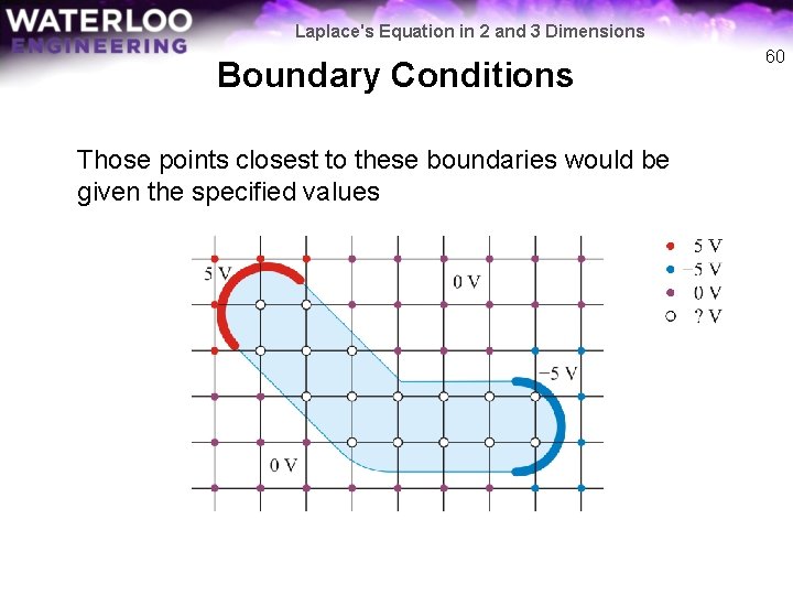
Laplace's Equation in 2 and 3 Dimensions Boundary Conditions Those points closest to these boundaries would be given the specified values 60

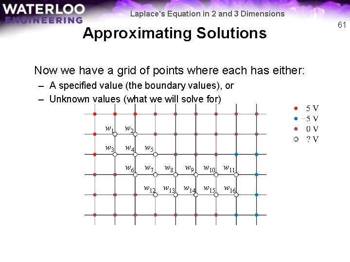
Laplace's Equation in 2 and 3 Dimensions Approximating Solutions Now we have a grid of points where each has either: – A specified value (the boundary values), or – Unknown values (what we will solve for) w 1 w 2 w 3 w 4 w 5 w 6 w 7 w 8 w 9 w 10 w 11 w 12 w 13 w 14 w 15 w 16 61

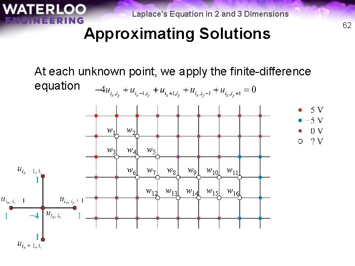
Laplace's Equation in 2 and 3 Dimensions Approximating Solutions At each unknown point, we apply the finite-difference equation w 1 w 2 w 3 w 4 w 5 w 6 w 7 w 8 w 9 w 10 w 11 w 12 w 13 w 14 w 15 w 16 62

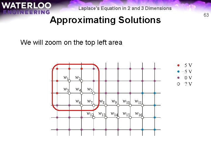
Laplace's Equation in 2 and 3 Dimensions Approximating Solutions We will zoom on the top left area w 1 w 2 w 3 w 4 w 5 w 6 w 7 w 8 w 9 w 10 w 11 w 12 w 13 w 14 w 15 w 16 63

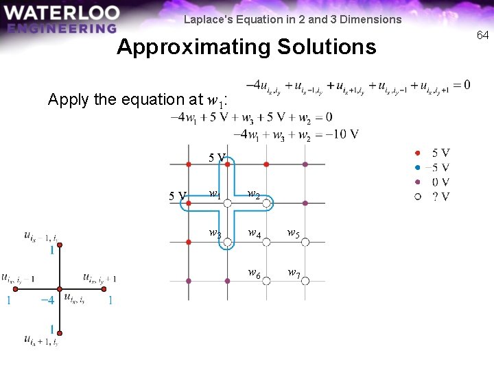
Laplace's Equation in 2 and 3 Dimensions Approximating Solutions Apply the equation at w 1: 5 V 5 V w 1 w 2 w 3 w 4 w 5 w 6 w 7 64

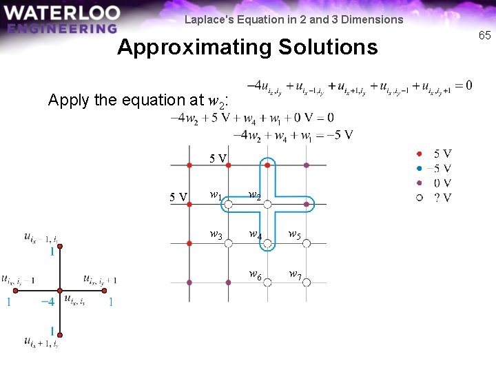
Laplace's Equation in 2 and 3 Dimensions Approximating Solutions Apply the equation at w 2: 5 V 5 V w 1 w 2 w 3 w 4 w 5 w 6 w 7 65

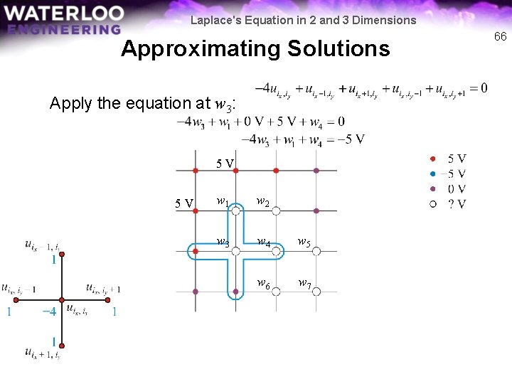
Laplace's Equation in 2 and 3 Dimensions Approximating Solutions Apply the equation at w 3: 5 V 5 V w 1 w 2 w 3 w 4 w 5 w 6 w 7 66

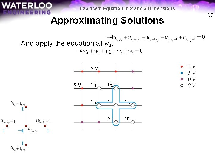
Laplace's Equation in 2 and 3 Dimensions Approximating Solutions And apply the equation at w 4: 5 V 5 V w 1 w 2 w 3 w 4 w 5 w 6 w 7 67

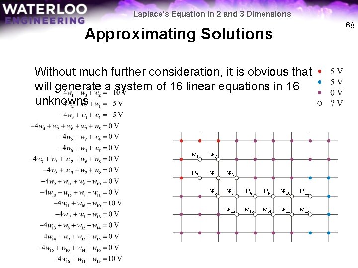
Laplace's Equation in 2 and 3 Dimensions 68 Approximating Solutions Without much further consideration, it is obvious that this will generate a system of 16 linear equations in 16 unknowns w 1 w 2 w 3 w 4 w 5 w 6 w 7 w 8 w 9 w 10 w 11 w 12 w 13 w 14 w 15 w 16

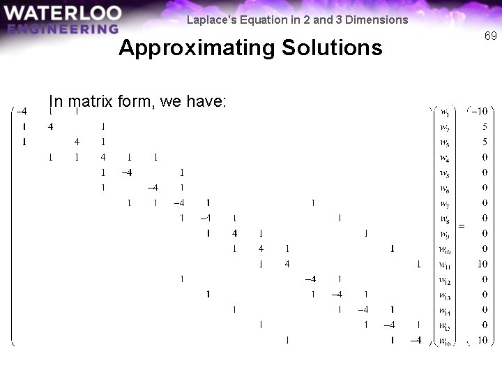
Laplace's Equation in 2 and 3 Dimensions Approximating Solutions In matrix form, we have: 69

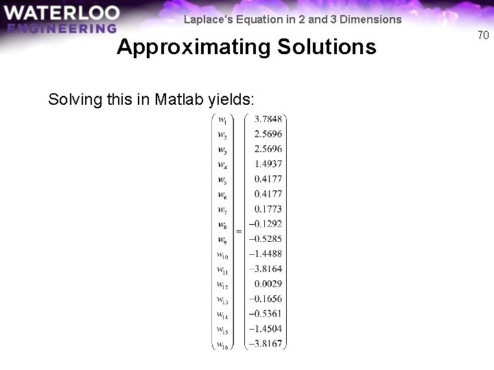
Laplace's Equation in 2 and 3 Dimensions Approximating Solutions Solving this in Matlab yields: 70

Laplace's Equation in 2 and 3 Dimensions Approximating Solutions Recall our initial designations of the 16 points: w 1 w 2 w 3 w 4 w 5 w 6 w 7 w 8 w 9 w 10 w 11 w 12 w 13 w 14 w 15 w 16 71

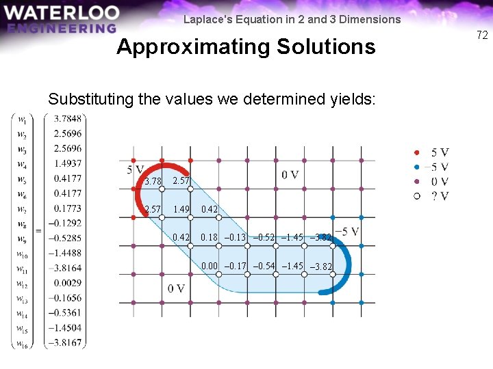
Laplace's Equation in 2 and 3 Dimensions Approximating Solutions Substituting the values we determined yields: 3. 78 2. 57 1. 49 0. 42 0. 18 – 0. 13 – 0. 52 – 1. 45 – 3. 82 0. 00 – 0. 17 – 0. 54 – 1. 45 – 3. 82 72

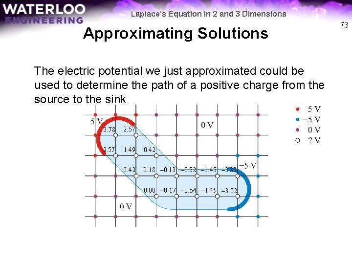
Laplace's Equation in 2 and 3 Dimensions Approximating Solutions The electric potential we just approximated could be used to determine the path of a positive charge from the source to the sink 3. 78 2. 57 1. 49 0. 42 0. 18 – 0. 13 – 0. 52 – 1. 45 – 3. 82 0. 00 – 0. 17 – 0. 54 – 1. 45 – 3. 82 73

Laplace's Equation in 2 and 3 Dimensions Approximating Insulated Boundaries If a boundary is insulated, we will assume it has a value equal to its neighbour 74

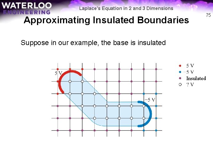
Laplace's Equation in 2 and 3 Dimensions Approximating Insulated Boundaries 75 Suppose in our example, the base is insulated Insulated

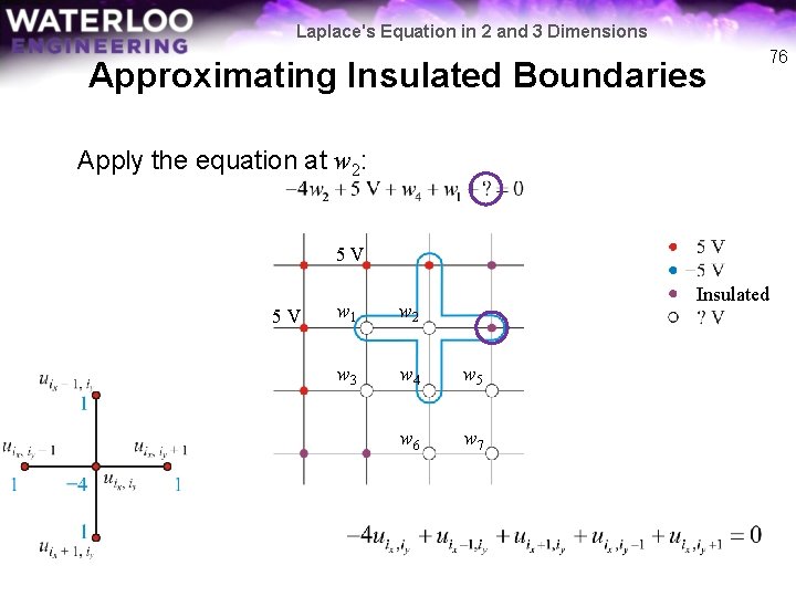
Laplace's Equation in 2 and 3 Dimensions Approximating Insulated Boundaries 76 Apply the equation at w 2: 5 V 5 V Insulated w 1 w 2 w 3 w 4 w 5 w 6 w 7

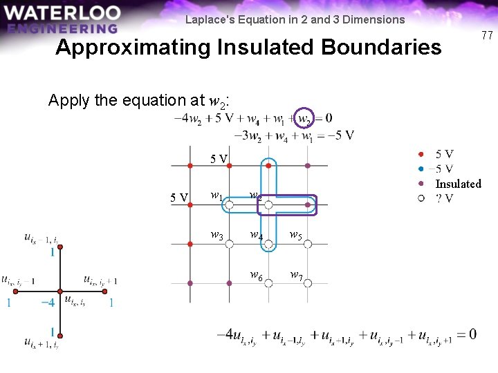
Laplace's Equation in 2 and 3 Dimensions Approximating Insulated Boundaries 77 Apply the equation at w 2: 5 V 5 V Insulated w 1 w 2 w 3 w 4 w 5 w 6 w 7

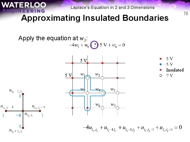
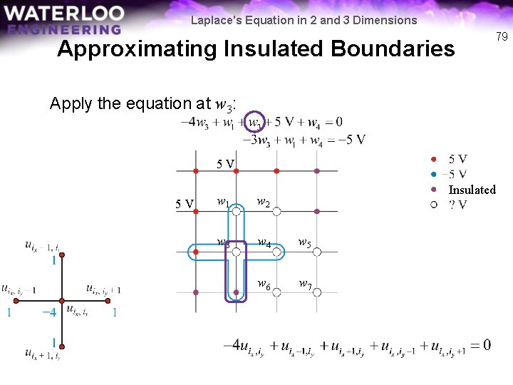
Laplace's Equation in 2 and 3 Dimensions Approximating Insulated Boundaries 78 Apply the equation at w 3: 5 V 5 V Insulated w 1 w 2 w 3 w 4 w 5 w 6 w 7

Laplace's Equation in 2 and 3 Dimensions Approximating Insulated Boundaries 79 Apply the equation at w 3: 5 V 5 V Insulated w 1 w 2 w 3 w 4 w 5 w 6 w 7

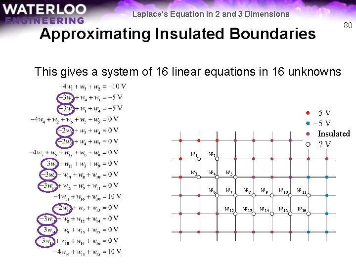
Laplace's Equation in 2 and 3 Dimensions 80 Approximating Insulated Boundaries This gives a system of 16 linear equations in 16 unknowns Insulated w 1 w 2 w 3 w 4 w 5 w 6 w 7 w 8 w 9 w 10 w 11 w 12 w 13 w 14 w 15 w 16

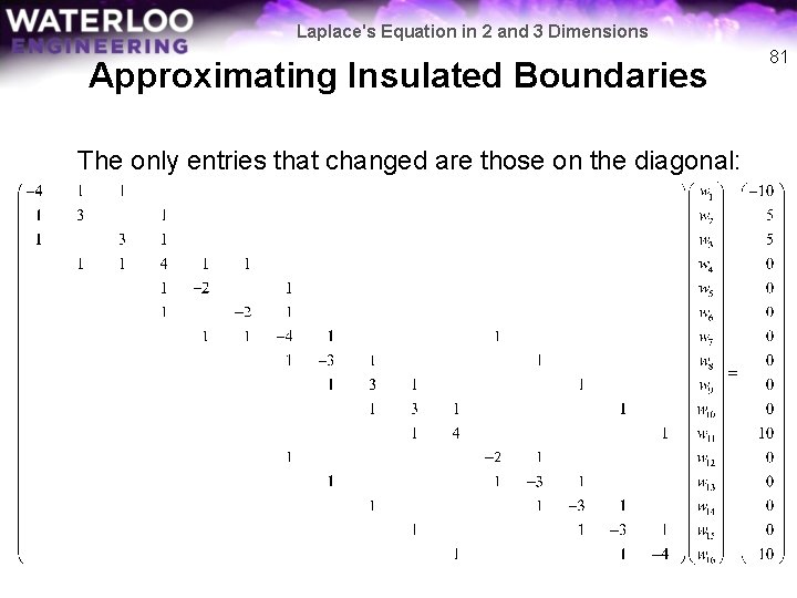
Laplace's Equation in 2 and 3 Dimensions Approximating Insulated Boundaries The only entries that changed are those on the diagonal: 81

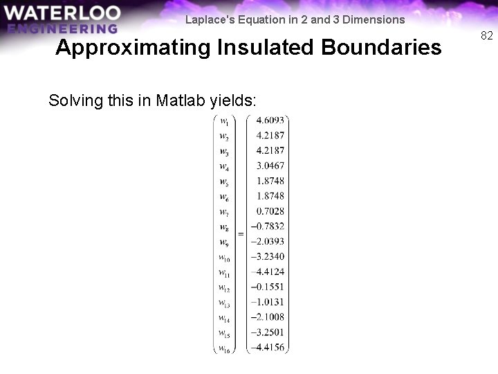
Laplace's Equation in 2 and 3 Dimensions Approximating Insulated Boundaries Solving this in Matlab yields: 82

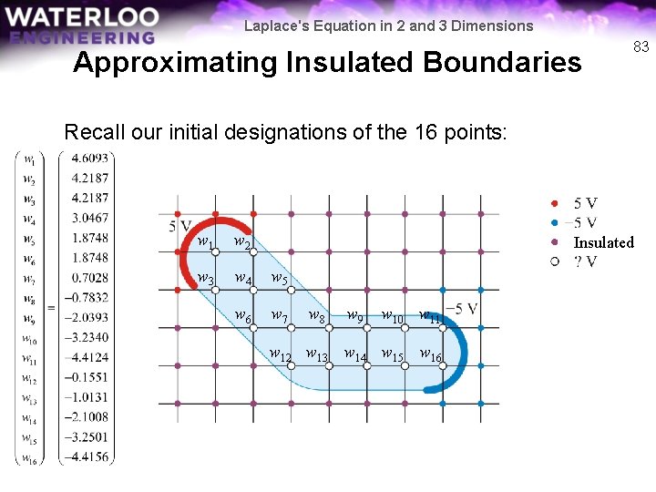
Laplace's Equation in 2 and 3 Dimensions Approximating Insulated Boundaries 83 Recall our initial designations of the 16 points: w 1 w 2 w 3 w 4 w 5 w 6 w 7 Insulated w 8 w 9 w 10 w 11 w 12 w 13 w 14 w 15 w 16

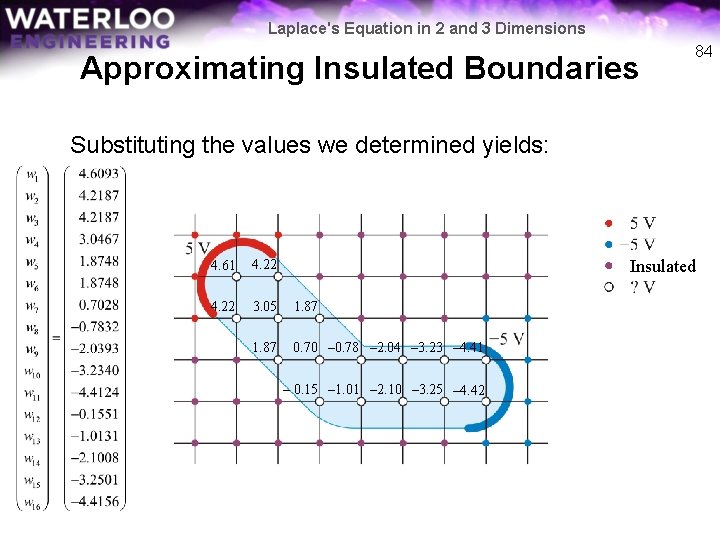
Laplace's Equation in 2 and 3 Dimensions Approximating Insulated Boundaries 84 Substituting the values we determined yields: Insulated 4. 61 4. 22 3. 05 1. 87 0. 70 – 0. 78 – 2. 04 – 3. 23 – 4. 41 – 0. 15 – 1. 01 – 2. 10 – 3. 25 – 4. 42

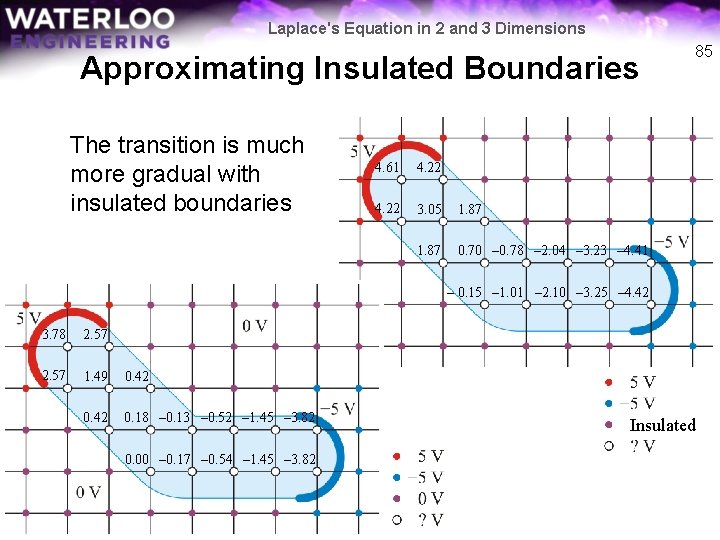
Laplace's Equation in 2 and 3 Dimensions Approximating Insulated Boundaries The transition is much more gradual with insulated boundaries 4. 61 4. 22 3. 05 1. 87 0. 70 – 0. 78 – 2. 04 – 3. 23 – 4. 41 85 – 0. 15 – 1. 01 – 2. 10 – 3. 25 – 4. 42 3. 78 2. 57 1. 49 0. 42 0. 18 – 0. 13 – 0. 52 – 1. 45 – 3. 82 0. 00 – 0. 17 – 0. 54 – 1. 45 – 3. 82 Insulated

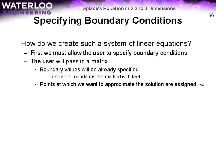
Laplace's Equation in 2 and 3 Dimensions Specifying Boundary Conditions How do we create such a system of linear equations? – First we must allow the user to specify boundary conditions – The user will pass in a matrix • Boundary values will be already specified – Insulated boundaries are marked with Na. N • Points at which we want to approximate the solution are assigned –∞ 86

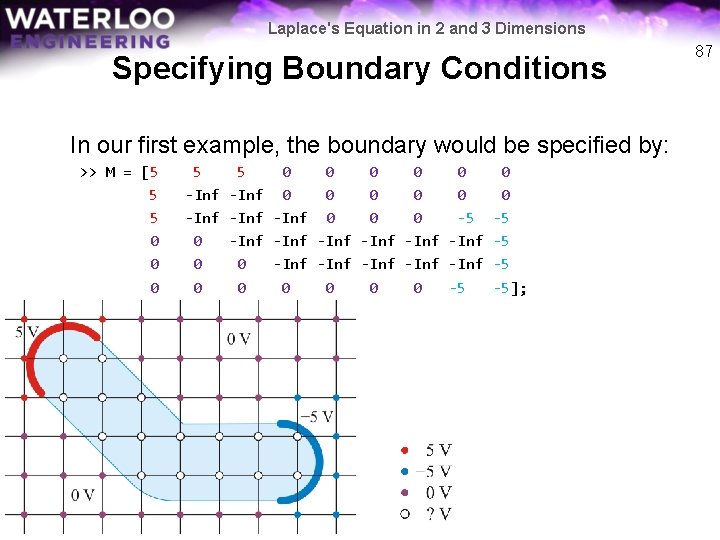
Laplace's Equation in 2 and 3 Dimensions Specifying Boundary Conditions In our first example, the boundary would be specified by: >> M = [5 5 5 0 0 0 -Inf 0 0 0 -Inf 0 0 0 -5 -5 0 -Inf -Inf -Inf -5 0 0 0 -5 -5]; 87

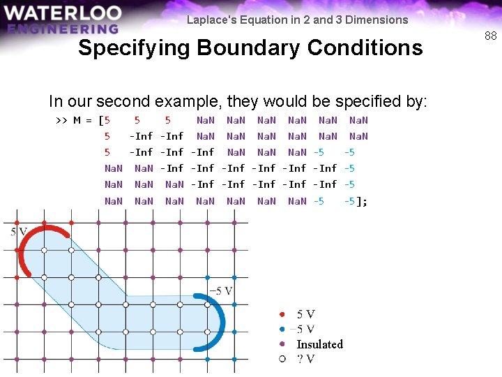
Laplace's Equation in 2 and 3 Dimensions Specifying Boundary Conditions In our second example, they would be specified by: >> M = [5 5 5 Na. N Na. N 5 -Inf -Inf Na. N -5 Na. N -Inf -Inf Na. N Na. N -5 Insulated Na. N -5 -5]; 88

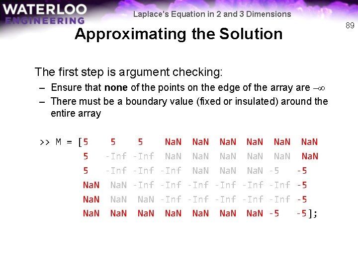
Laplace's Equation in 2 and 3 Dimensions 89 Approximating the Solution The first step is argument checking: – Ensure that none of the points on the edge of the array are –∞ – There must be a boundary value (fixed or insulated) around the entire array >> M = [5 5 5 Na. N Na. N 5 -Inf -Inf Na. N -5 Na. N -Inf -Inf Na. N Na. N -5 -5];

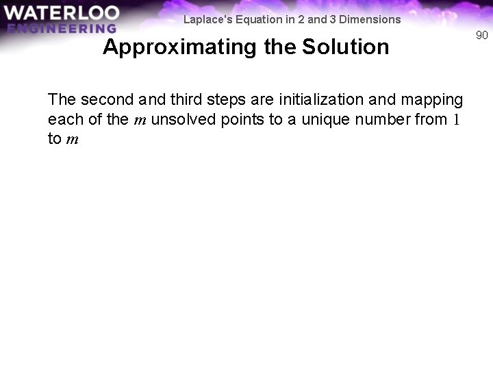
Laplace's Equation in 2 and 3 Dimensions Approximating the Solution The second and third steps are initialization and mapping each of the m unsolved points to a unique number from 1 to m 90

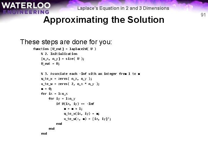
Laplace's Equation in 2 and 3 Dimensions Approximating the Solution These steps are done for you: function [U_out] = laplace 2 d( U ) % 2. Initialization [n_x, n_y] = size( U ); U_out = U; % 3. Associate each -Inf with an integer from 1 to m u_to_w = zeros( n_x, n_y ); w_to_u = zeros( 2, n_x * n_y ); m = 0; for ix = 1: n_x for iy = 1: n_y if U(ix, iy) == -Inf m = m + 1; u_to_w(ix, iy) = m; w_to_u(: , m) = [ix, iy]'; end end 91

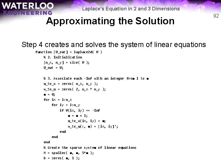
Laplace's Equation in 2 and 3 Dimensions Approximating the Solution Step 4 creates and solves the system of linear equations function [U_out] = laplace 2 d( U ) % 2. Initialization [n_x, n_y] = size( U ); U_out = U; % 3. Associate each -Inf with an integer from 1 to m u_to_w = zeros( n_x, n_y ); w_to_u = zeros( 2, n_x * n_y ); m = 0; for ix = 1: n_x for iy = 1: n_y if U(ix, iy) == -Inf m = m + 1; u_to_w(ix, iy) = m; w_to_u(: , m) = [ix, iy]'; end end % Create the sparse system of linear equations M = spalloc( m, m, 5*m ); b = zeros( m, 1 ); 92

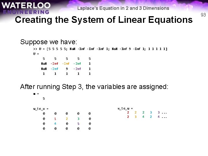
Laplace's Equation in 2 and 3 Dimensions Creating the System of Linear Equations Suppose we have: >> U = [5 5 5; Na. N -Inf 1; Na. N -Inf 9 -Inf 1; 1 1 1] U = 5 5 5 Na. N -Inf 1 Na. N -Inf 9 -Inf 1 1 1 After running Step 3, the variables are assigned: m = 5 u_to_w = 0 0 0 1 4 0 0 2 0 0 0 3 5 0 0 0 w_to_u = 2 2 2 3 2 4 3 2 3. . . 4. . . 93

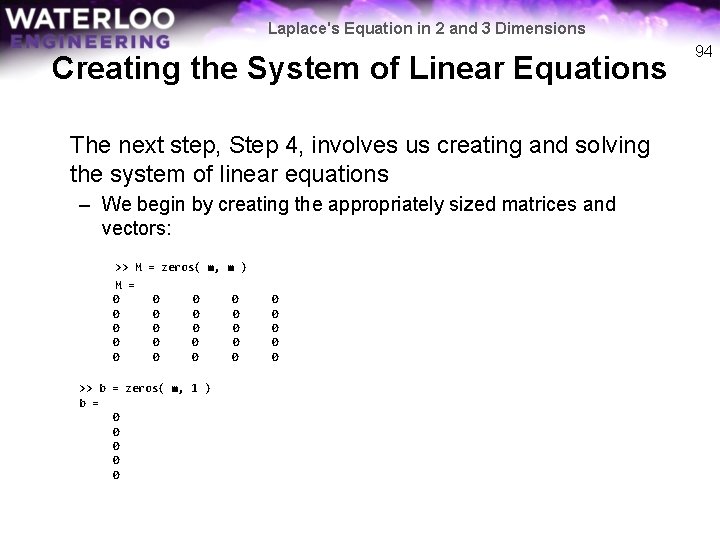
Laplace's Equation in 2 and 3 Dimensions Creating the System of Linear Equations The next step, Step 4, involves us creating and solving the system of linear equations – We begin by creating the appropriately sized matrices and vectors: >> M M = 0 0 0 = zeros( m, m ) 0 0 0 0 0 >> b = zeros( m, 1 ) b = 0 0 0 0 94

Laplace's Equation in 2 and 3 Dimensions Creating the System of Linear Equations How do we update M and b? 95

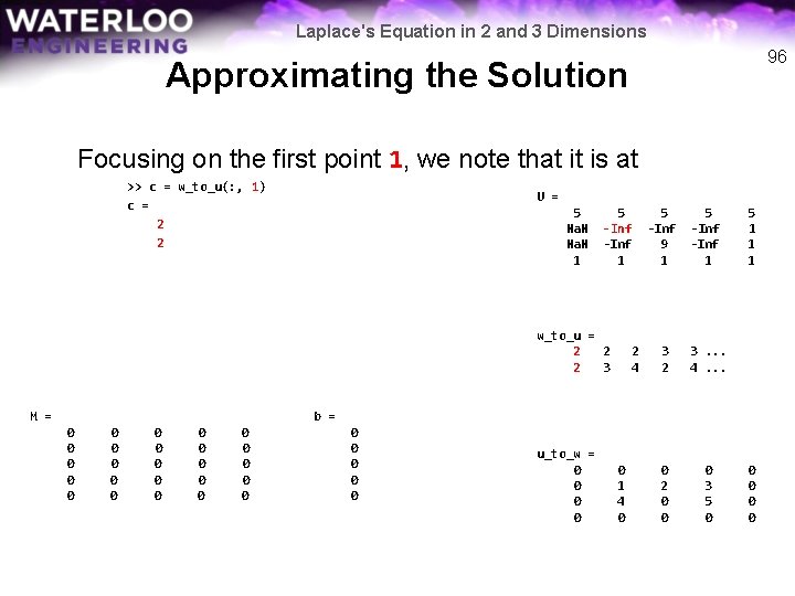
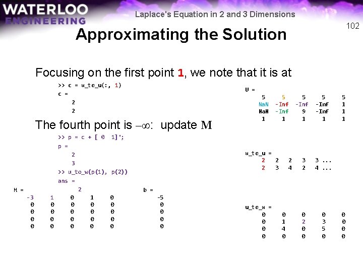
Laplace's Equation in 2 and 3 Dimensions 96 Approximating the Solution Focusing on the first point 1, we note that it is at >> c = w_to_u(: , 1) c = 2 2 U = 5 Na. N 1 5 -Inf 1 w_to_u = 2 2 2 3 M = 5 -Inf 9 1 2 4 5 -Inf 1 3 2 3. . . 4. . . 0 2 0 0 0 3 5 0 5 1 1 1 b = 0 0 0 0 0 0 0 0 u_to_w = 0 0 0 1 4 0 0 0

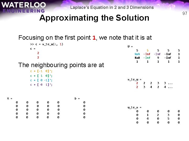
Laplace's Equation in 2 and 3 Dimensions 97 Approximating the Solution Focusing on the first point 1, we note that it is at >> c = w_to_u(: , 1) c = 2 2 U = The neighbouring points are at c c + + [-1 0]'; [ 0 -1]'; [ 0 1]'; 5 Na. N 1 5 -Inf 1 w_to_u = 2 2 2 3 M = 2 4 5 -Inf 9 1 5 -Inf 1 3 2 3. . . 4. . . 0 2 0 0 0 3 5 0 5 1 1 1 b = 0 0 0 0 0 0 0 0 u_to_w = 0 0 0 1 4 0 0 0

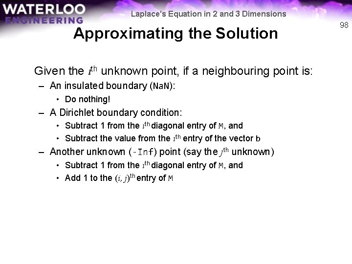
Laplace's Equation in 2 and 3 Dimensions Approximating the Solution Given the ith unknown point, if a neighbouring point is: – An insulated boundary (Na. N): • Do nothing! – A Dirichlet boundary condition: • Subtract 1 from the ith diagonal entry of M, and • Subtract the value from the ith entry of the vector b – Another unknown (-Inf) point (say the jth unknown) • Subtract 1 from the ith diagonal entry of M, and • Add 1 to the (i, j)th entry of M 98

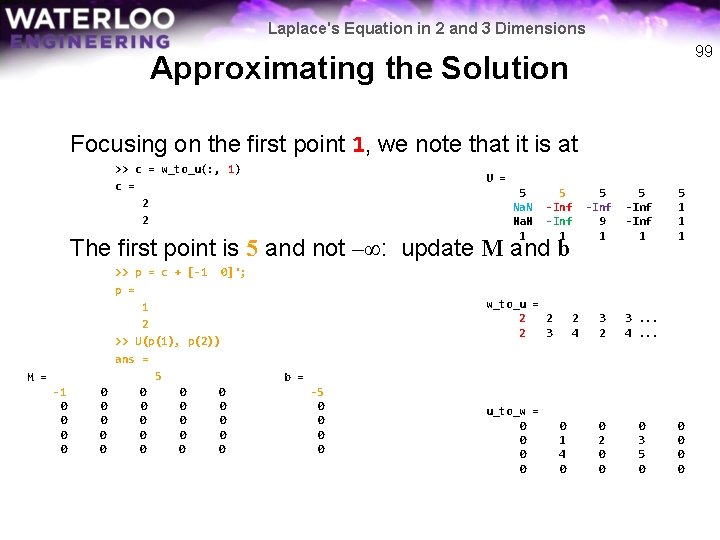
Laplace's Equation in 2 and 3 Dimensions 99 Approximating the Solution Focusing on the first point 1, we note that it is at >> c = w_to_u(: , 1) c = 2 2 U = 5 Na. N 1 5 -Inf 1 The first point is 5 and not –∞: update M and b M = -1 0 0 0 0 0 >> p = c + [-1 0]'; p = 1 2 >> U(p(1), p(2)) ans = 5 0 0 0 0 w_to_u = 2 2 2 3 2 4 5 -Inf 9 1 5 -Inf 1 3 2 3. . . 4. . . 0 2 0 0 0 3 5 0 5 1 1 1 b = -5 0 0 u_to_w = 0 0 0 1 4 0 0 0

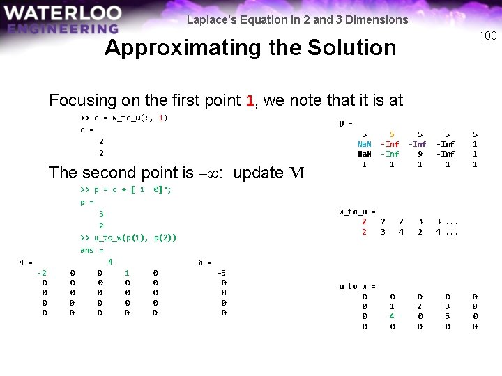
Laplace's Equation in 2 and 3 Dimensions 100 Approximating the Solution Focusing on the first point 1, we note that it is at >> c = w_to_u(: , 1) c = 2 2 U = The second point is –∞: update M M = -2 0 0 0 0 0 >> p = c + [ 1 p = 3 2 >> u_to_w(p(1), ans = 4 0 1 0 0 0 0 5 Na. N 1 5 -Inf 9 1 5 -Inf 1 3 2 3. . . 4. . . 0 2 0 0 0 3 5 0 5 1 1 1 0]'; w_to_u = 2 2 2 3 p(2)) 2 4 b = 0 0 0 -5 0 0 u_to_w = 0 0 0 1 4 0 0 0

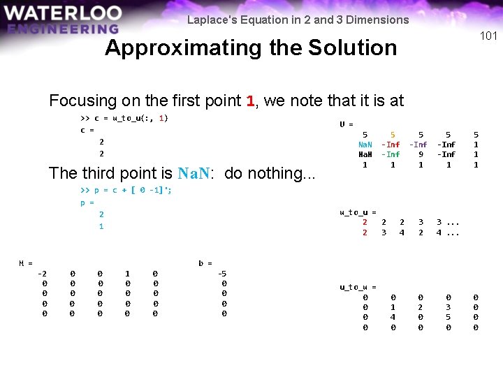
Laplace's Equation in 2 and 3 Dimensions 101 Approximating the Solution Focusing on the first point 1, we note that it is at >> c = w_to_u(: , 1) c = 2 2 U = The third point is Na. N: do nothing. . . >> p = c + [ 0 -1]'; p = 2 1 M = 5 Na. N 1 5 -Inf 1 w_to_u = 2 2 2 3 2 4 5 -Inf 9 1 5 -Inf 1 3 2 3. . . 4. . . 0 2 0 0 0 3 5 0 5 1 1 1 b = -2 0 0 0 0 1 0 0 0 0 0 -5 0 0 u_to_w = 0 0 0 1 4 0 0 0

Laplace's Equation in 2 and 3 Dimensions 102 Approximating the Solution Focusing on the first point 1, we note that it is at >> c = w_to_u(: , 1) c = 2 2 U = The fourth point is –∞: update M M = -3 0 0 1 0 0 >> p = c + [ 0 p = 2 3 >> u_to_w(p(1), ans = 2 0 1 0 0 0 0 5 Na. N 1 5 -Inf 9 1 5 -Inf 1 3 2 3. . . 4. . . 0 2 0 0 0 3 5 0 5 1 1]'; w_to_u = 2 2 2 3 p(2)) 2 4 b = 0 0 0 -5 0 0 u_to_w = 0 0 0 1 4 0 0 0

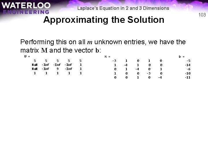
Laplace's Equation in 2 and 3 Dimensions 103 Approximating the Solution Performing this on all m unknown entries, we have the matrix M and the vector b: U = 5 Na. N 1 5 -Inf 9 1 5 -Inf 1 5 1 1 1 M = b = -3 1 0 1 -4 1 0 0 0 1 -4 0 1 1 0 0 -3 0 0 0 1 0 -4 -5 -14 -6 -10 -11

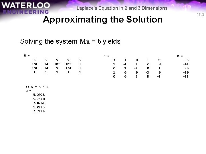
Laplace's Equation in 2 and 3 Dimensions 104 Approximating the Solution Solving the system Mu = b yields U = 5 Na. N 1 5 -Inf 1 >> u = M b u = 5. 2978 5. 7940 3. 8784 5. 0993 3. 7196 5 -Inf 9 1 5 -Inf 1 5 1 1 1 M = b = -3 1 0 1 -4 1 0 0 0 1 -4 0 1 1 0 0 -3 0 0 0 1 0 -4 -5 -14 -6 -10 -11

Laplace's Equation in 2 and 3 Dimensions 105 Approximating the Solution Step 5 has us substitute these values back into Uout: U = 5 Na. N 1 5 -Inf 1 >> u = M b u = 5. 2978 5. 7940 3. 8784 5. 0993 3. 7196 5 -Inf 9 1 5 -Inf 1 M = 5 1 1 1 b = -3 1 0 U_out = 5. 0000 Na. N 1. 0000 1 -4 1 0 0 5. 0000 5. 2978 5. 0993 1. 0000 w_to_u = 2 2 2 3 2 4 0 1 -4 0 1 5. 0000 5. 7940 9. 0000 1. 0000 3 2 3. . . 4. . . 1 0 0 -3 0 5. 0000 3. 8784 3. 7196 1. 0000 0 0 1 0 -4 -5 -14 -6 -10 -11 5. 0000 1. 0000

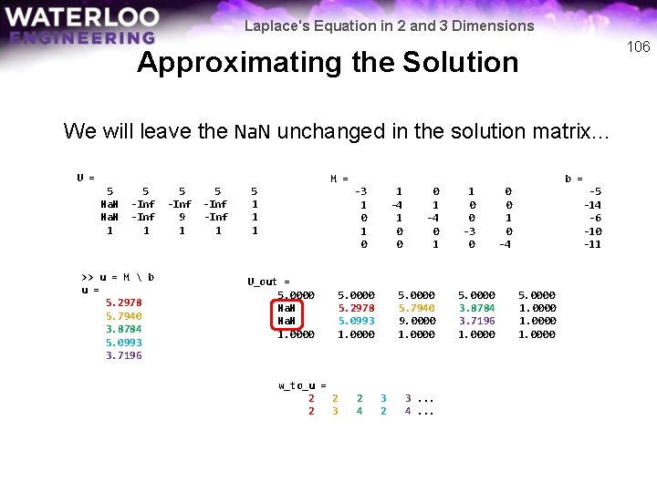
Laplace's Equation in 2 and 3 Dimensions 106 Approximating the Solution We will leave the Na. N unchanged in the solution matrix. . . U = 5 Na. N 1 5 -Inf 1 >> u = M b u = 5. 2978 5. 7940 3. 8784 5. 0993 3. 7196 5 -Inf 9 1 5 -Inf 1 M = 5 1 1 1 b = -3 1 0 U_out = 5. 0000 Na. N 1. 0000 1 -4 1 0 0 5. 0000 5. 2978 5. 0993 1. 0000 w_to_u = 2 2 2 3 2 4 0 1 -4 0 1 5. 0000 5. 7940 9. 0000 1. 0000 3 2 3. . . 4. . . 1 0 0 -3 0 5. 0000 3. 8784 3. 7196 1. 0000 0 0 1 0 -4 -5 -14 -6 -10 -11 5. 0000 1. 0000

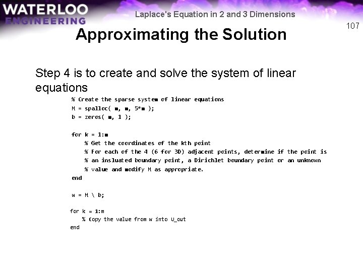
Laplace's Equation in 2 and 3 Dimensions Approximating the Solution Step 4 is to create and solve the system of linear equations % Create the sparse system of linear equations M = spalloc( m, m, 5*m ); b = zeros( m, 1 ); for k % % end = 1: m Get the coordinates of the kth point For each of the 4 (6 for 3 D) adjacent points, determine if the point is an insluated boundary point, a Dirichlet boundary point or an unknown value and modify M as appropriate. w = M b; for k = 1: m % Copy the value from w into U_out end 107

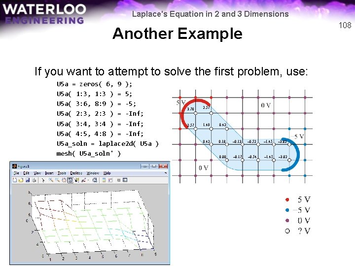
Laplace's Equation in 2 and 3 Dimensions 108 Another Example If you want to attempt to solve the first problem, use: U 5 a = zeros( 6, 9 ); U 5 a( 1: 3, 1: 3 ) = 5; U 5 a( 3: 6, 8: 9 ) = -5; U 5 a( 2: 3, 2: 3 ) = -Inf; U 5 a( 3: 4, 3: 4 ) = -Inf; U 5 a( 4: 5, 4: 8 ) = -Inf; U 5 a_soln = laplace 2 d( U 5 a ) mesh( U 5 a_soln' ) 3. 78 2. 57 1. 49 0. 42 0. 18 – 0. 13 – 0. 52 – 1. 45 – 3. 82 0. 00 – 0. 17 – 0. 54 – 1. 45 – 3. 82

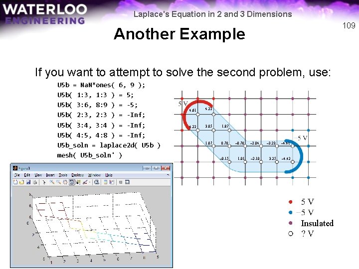
Laplace's Equation in 2 and 3 Dimensions 109 Another Example If you want to attempt to solve the second problem, use: U 5 b = Na. N*ones( 6, 9 ); U 5 b( 1: 3, 1: 3 ) = 5; U 5 b( 3: 6, 8: 9 ) = -5; U 5 b( 2: 3, 2: 3 ) = -Inf; U 5 b( 3: 4, 3: 4 ) = -Inf; U 5 b( 4: 5, 4: 8 ) = -Inf; U 5 b_soln = laplace 2 d( U 5 b ) mesh( U 5 b_soln' ) 4. 61 4. 22 3. 05 1. 87 0. 70 – 0. 78 – 2. 04 – 3. 23 – 4. 41 – 0. 15 1. 01 – 2. 10 3. 25 – 4. 42 Insulated

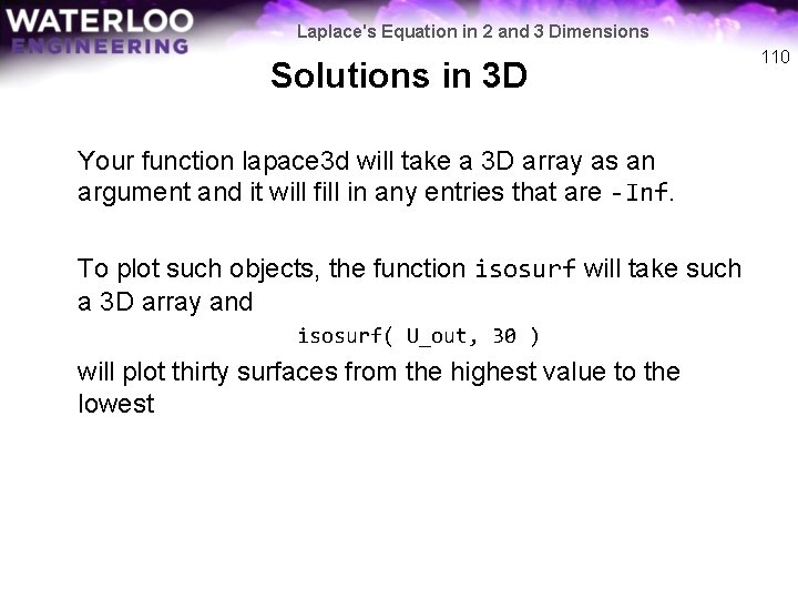
Laplace's Equation in 2 and 3 Dimensions Solutions in 3 D Your function lapace 3 d will take a 3 D array as an argument and it will fill in any entries that are -Inf. To plot such objects, the function isosurf will take such a 3 D array and isosurf( U_out, 30 ) will plot thirty surfaces from the highest value to the lowest 110

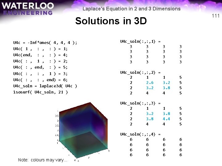
Laplace's Equation in 2 and 3 Dimensions 111 Solutions in 3 D U 4 c = -Inf*ones( 4, 4, 4 ); U 4 c( 1 , : ) = 1; U 4 c(end, : ) = 4; U 4 c( : , 1 , : ) = 2; U 4 c( : , end, : ) = 5; U 4 c( : , 1 ) = 3; U 4 c( : , end) = 6; U 4 c_soln = laplace 3 d( U 4 c ) isosurf( U 4 c_soln, 21 ) Note: colours may vary. . . U 4 c_soln(: , 1) = 3 3 3 3 U 4 c_soln(: , 2) = 2 1 1 2 2. 6 3. 2 2 3. 8 2 4 4 5 5 U 4 c_soln(: , 3) = 2 1 1 2 3. 8 4. 4 2 4 4 5 5 U 4 c_soln(: , 4) = 6 6 6 6

Laplace's Equation in 2 and 3 Dimensions 112 Solutions in 3 D U 4 d = -Inf*ones( 15, 15 ); U 4 d([1, end], : ) = 100; U 4 d(: , [1, end], : ) = 0; U 4 d(: , [1, end]) = 0; U 4 d_soln = laplace 3 d( U 4 d ) isosurf( U 4 d_soln, 21 ) Note: isosurf is available for download in the Laboratory directory Note: colours may vary. . .

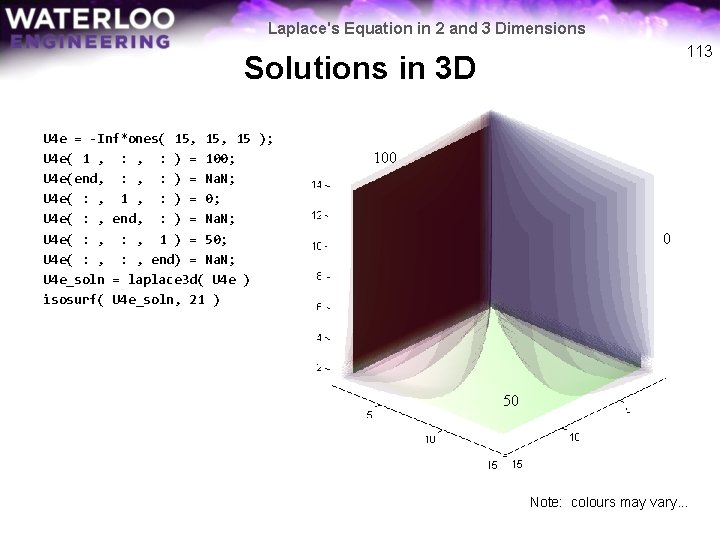
Laplace's Equation in 2 and 3 Dimensions 113 Solutions in 3 D U 4 e = -Inf*ones( 15, 15 ); U 4 e( 1 , : ) = 100; U 4 e(end, : ) = Na. N; U 4 e( : , 1 , : ) = 0; U 4 e( : , end, : ) = Na. N; U 4 e( : , 1 ) = 50; U 4 e( : , end) = Na. N; U 4 e_soln = laplace 3 d( U 4 e ) isosurf( U 4 e_soln, 21 ) 100 0 50 Note: colours may vary. . .

Laplace's Equation in 2 and 3 Dimensions 114 Solutions in 3 D U 4 f = -Inf*ones( 15, 15 ); U 4 f([1, end], : ) = Na. N; U 4 f(: , 1) = 0; U 4 f(: , end) = Na. N; U 4 f(8, 8, 8) = 100; U 4 f_soln = laplace 3 d( U 4 f ) isosurf( U 4 f_soln, 100 ) 16 33 10 Note: colours may vary. . .

Laplace's Equation in 2 and 3 Dimensions Laboratory 5 During the laboratory, you will implement two functions: lapace 2 d and laplace 3 d Once you have lapace 2 d working, laplace 3 d will require only a few modifications 115

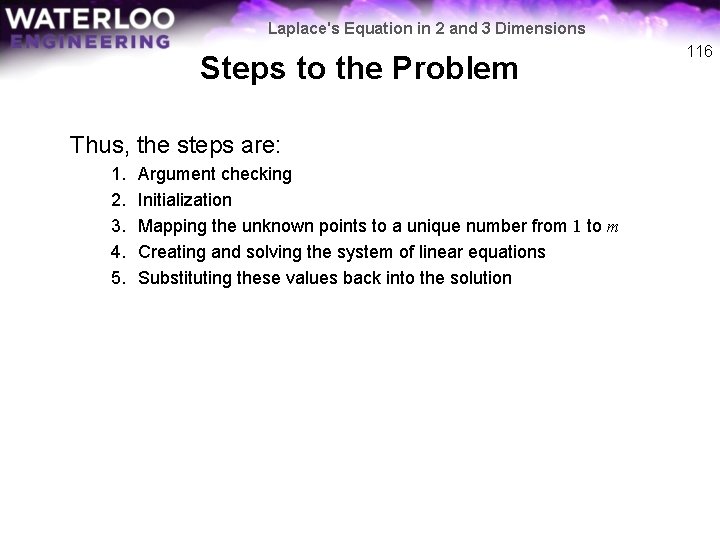
Laplace's Equation in 2 and 3 Dimensions Steps to the Problem Thus, the steps are: 1. 2. 3. 4. 5. Argument checking Initialization Mapping the unknown points to a unique number from 1 to m Creating and solving the system of linear equations Substituting these values back into the solution 116

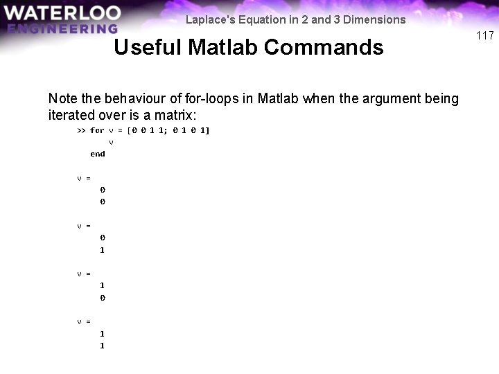
Laplace's Equation in 2 and 3 Dimensions Useful Matlab Commands Note the behaviour of for-loops in Matlab when the argument being iterated over is a matrix: >> for v = [0 0 1 1; 0 1] v end v = 0 0 v = 0 1 v = 1 0 v = 1 1 117

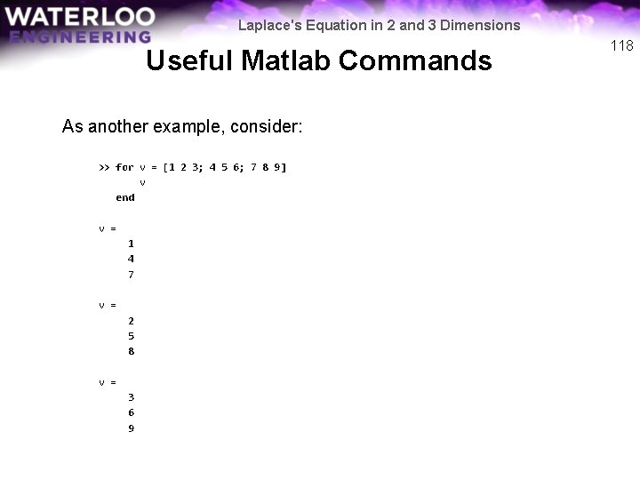
Laplace's Equation in 2 and 3 Dimensions Useful Matlab Commands As another example, consider: >> for v = [1 2 3; 4 5 6; 7 8 9] v end v = 1 4 7 v = 2 5 8 v = 3 6 9 118

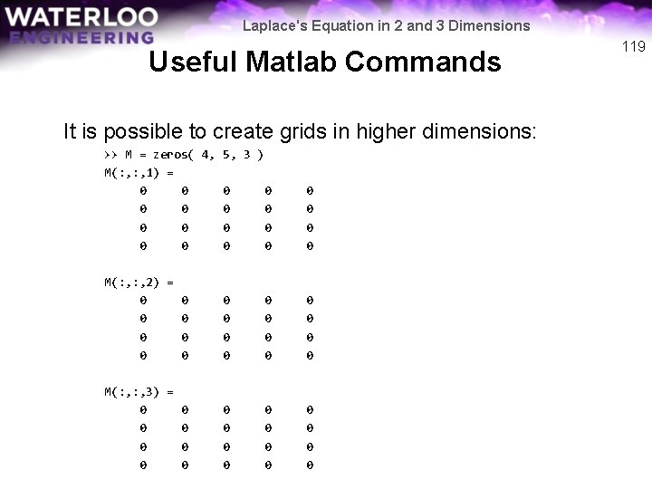
Laplace's Equation in 2 and 3 Dimensions Useful Matlab Commands It is possible to create grids in higher dimensions: >> M = zeros( 4, 5, 3 ) M(: , 1) = 0 0 0 0 0 M(: , 2) = 0 0 0 0 0 M(: , 3) = 0 0 0 0 0 119

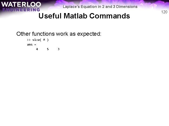
Laplace's Equation in 2 and 3 Dimensions Useful Matlab Commands Other functions work as expected: >> size( M ) ans = 4 5 3 120

Laplace's Equation in 2 and 3 Dimensions Useful Matlab Commands Matrices indexed by more than two indices have their dimensions checked using ndims: >> ndims( M ) ans = 3 >> ndims( 1 ) ans = 2 >> ndims( [1 2 3] ) ans = 2 >> ndims( [1 2 3 4; 5 6 7 8] ) ans = 2 121

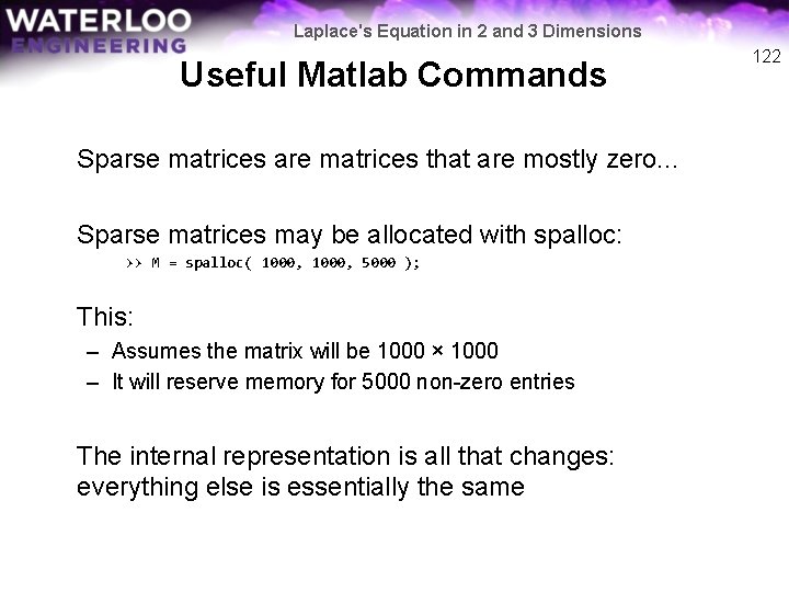
Laplace's Equation in 2 and 3 Dimensions Useful Matlab Commands Sparse matrices are matrices that are mostly zero. . . Sparse matrices may be allocated with spalloc: >> M = spalloc( 1000, 5000 ); This: – Assumes the matrix will be 1000 × 1000 – It will reserve memory for 5000 non-zero entries The internal representation is all that changes: everything else is essentially the same 122

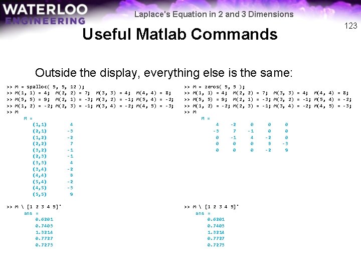
Laplace's Equation in 2 and 3 Dimensions 123 Useful Matlab Commands Outside the display, everything else is the same: >> >> >> M = spalloc( 5, 5, 12 M(1, 1) = 4; M(2, 2) M(5, 5) = 9; M(2, 1) M(1, 2) = -2; M(2, 3) M M = (1, 1) 4 (2, 1) -3 (1, 2) -2 (2, 2) 7 (3, 2) -1 (2, 3) -1 (3, 3) 4 (3, 4) -2 (4, 4) 8 (5, 4) -2 (4, 5) -3 (5, 5) 9 >> M [1 2 3 4 5]' ans = 0. 6201 0. 7403 1. 3214 0. 7727 0. 7273 ); = 7; M(3, 3) = 4; M(4, 4) = 8; = -3; M(3, 2) = -1; M(5, 4) = -2; = -1; M(3, 4) = -2; M(4, 5) = -3; >> >> >> M = zeros( 5, 5 ); M(1, 1) = 4; M(2, M(5, 5) = 9; M(2, M(1, 2) = -2; M(2, M M = 4 -2 -3 7 0 -1 0 0 >> M [1 2 3 4 5]' ans = 0. 6201 0. 7403 1. 3214 0. 7727 0. 7273 2) = 7; M(3, 3) = 4; M(4, 4) = 8; 1) = -3; M(3, 2) = -1; M(5, 4) = -2; 3) = -1; M(3, 4) = -2; M(4, 5) = -3; 0 -1 4 0 0 -2 8 -2 0 0 0 -3 9

Laplace's Equation in 2 and 3 Dimensions Summary We have looked at solving Laplace’s equation – Considered the physical problem for Laplace’s equation – Considered the effects in two and three dimensions – Found a finite-difference equation approximating Laplace’s equation in both two and three dimensions • We find those points that are unknown: 1, …, m • We set up the system of equations • We solve the system of equations and substitute the values back into the matrix 124

Laplace's Equation in 2 and 3 Dimensions References [1] Glyn James, Modern Engineering Mathematics, 4 th Ed. , Prentice Hall, 2007, p. 778. [2] Glyn James, Advanced Modern Engineering Mathematics, 4 th Ed. , Prentice Hall, 2011, p. 164. 125