LAPLACE TRANSFORMS PARTA UNITV LAPLACE TRANSFORM The Laplace

LAPLACE TRANSFORMS PART-A UNIT-V

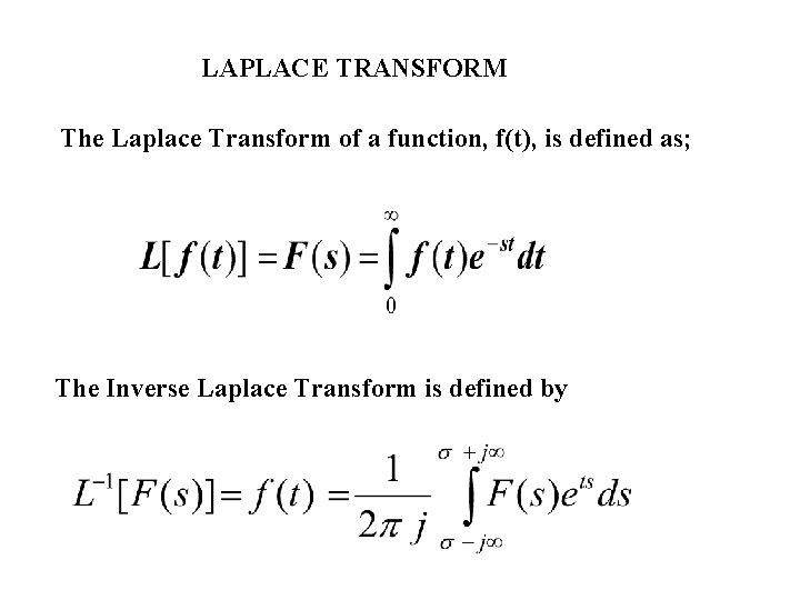
LAPLACE TRANSFORM The Laplace Transform of a function, f(t), is defined as; The Inverse Laplace Transform is defined by

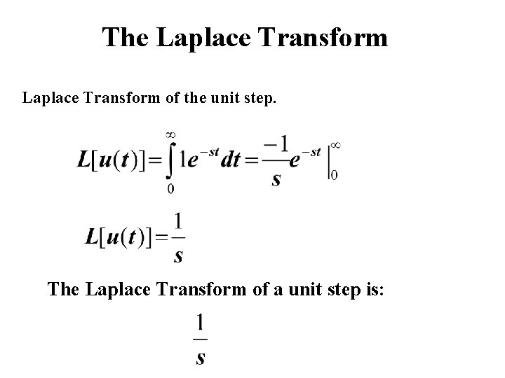
The Laplace Transform of the unit step. The Laplace Transform of a unit step is:

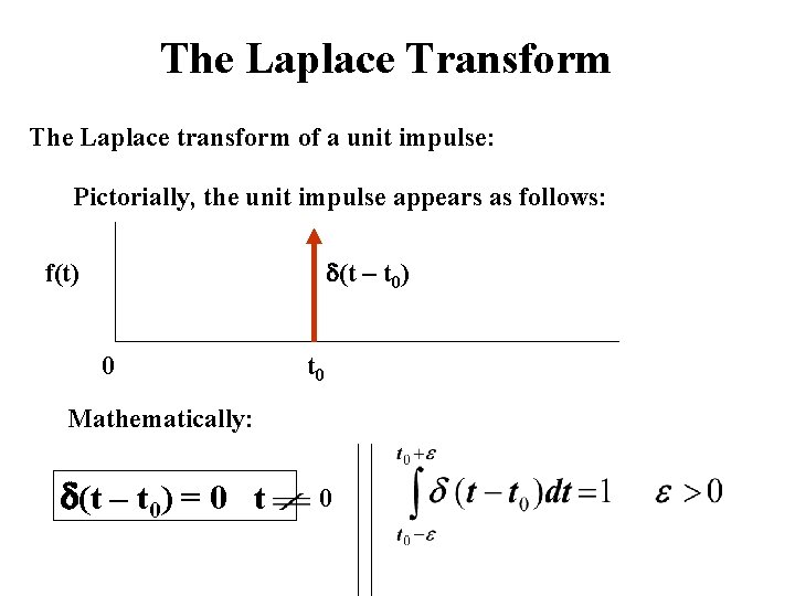
The Laplace Transform The Laplace transform of a unit impulse: Pictorially, the unit impulse appears as follows: (t – t 0) f(t) 0 t 0 Mathematically: (t – t 0) = 0 t 0

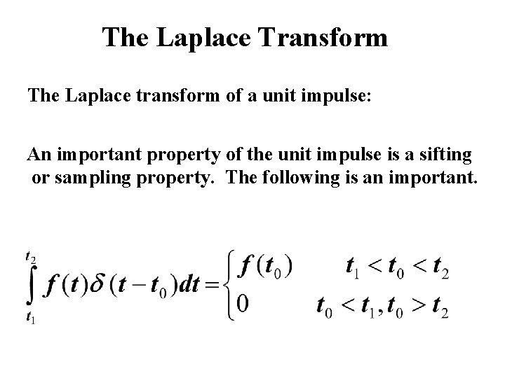
The Laplace Transform The Laplace transform of a unit impulse: An important property of the unit impulse is a sifting or sampling property. The following is an important.

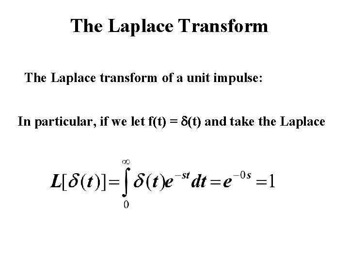
The Laplace Transform The Laplace transform of a unit impulse: In particular, if we let f(t) = (t) and take the Laplace

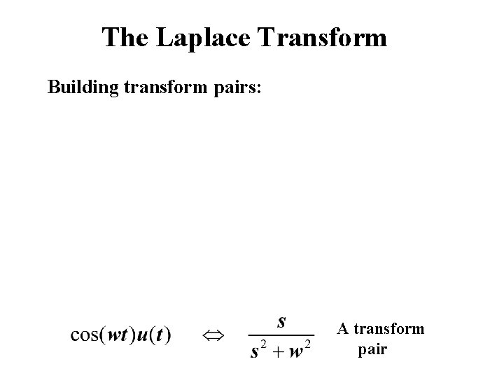
The Laplace Transform Building transform pairs: A transform pair

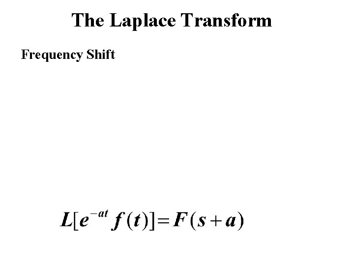
The Laplace Transform Frequency Shift

The Laplace Transform Time Integration: The property is:

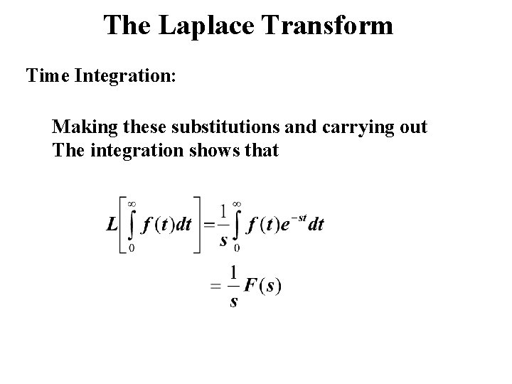
The Laplace Transform Time Integration: Making these substitutions and carrying out The integration shows that

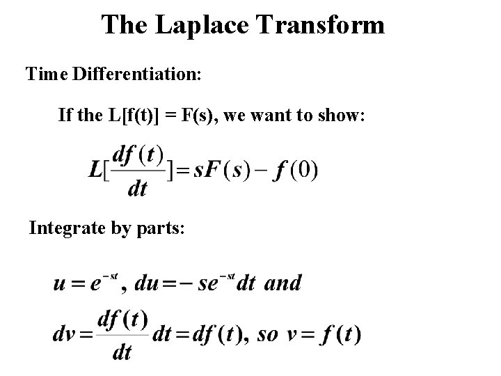
The Laplace Transform Time Differentiation: If the L[f(t)] = F(s), we want to show: Integrate by parts:

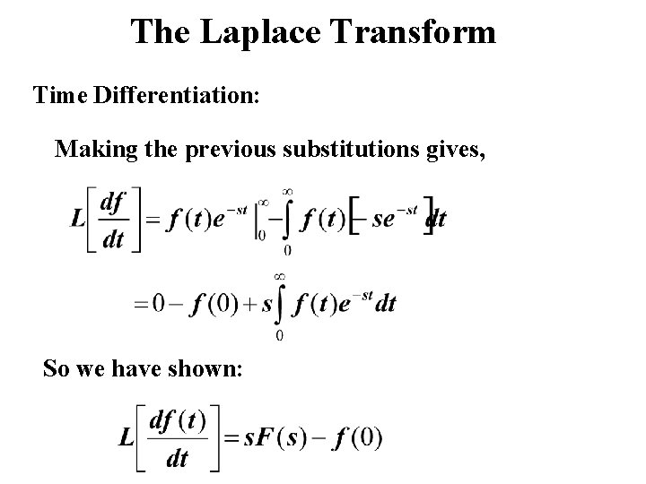
The Laplace Transform Time Differentiation: Making the previous substitutions gives, So we have shown:

The Laplace Transform Time Differentiation: We can extend the previous to show;

The Laplace Transform Pairs: f(t) F(s)

The Laplace Transform Pairs: f(t) F(s)

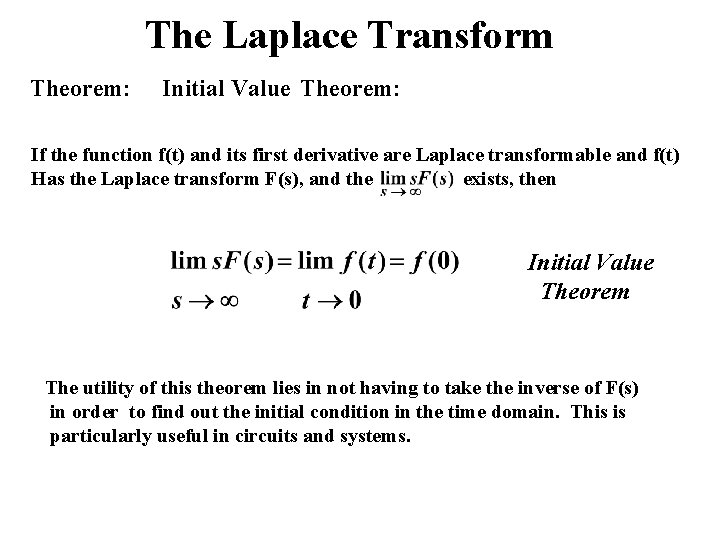
The Laplace Transform Theorem: Initial Value Theorem: If the function f(t) and its first derivative are Laplace transformable and f(t) Has the Laplace transform F(s), and the exists, then Initial Value Theorem The utility of this theorem lies in not having to take the inverse of F(s) in order to find out the initial condition in the time domain. This is particularly useful in circuits and systems.

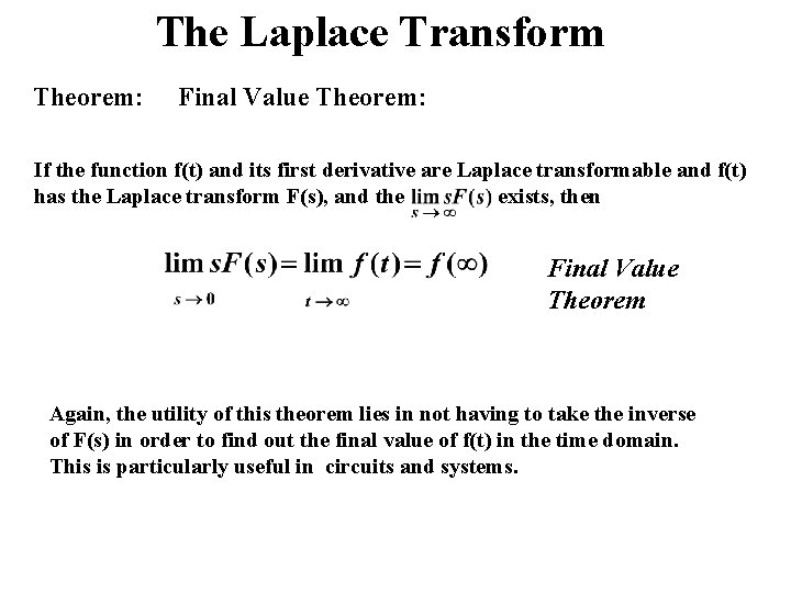
The Laplace Transform Theorem: Final Value Theorem: If the function f(t) and its first derivative are Laplace transformable and f(t) has the Laplace transform F(s), and the exists, then Final Value Theorem Again, the utility of this theorem lies in not having to take the inverse of F(s) in order to find out the final value of f(t) in the time domain. This is particularly useful in circuits and systems.

Why z-Transform? • A generalization of Fourier transform • Why generalize it? – FT does not converge on all sequence – Notation good for analysis – Bring the power of complex variable theory deal with the discrete-time signals and systems

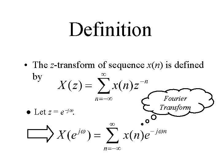
Definition • The z-transform of sequence x(n) is defined by l Let z = e j. Fourier Transform

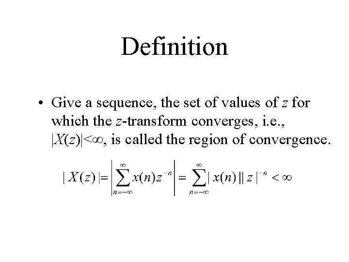
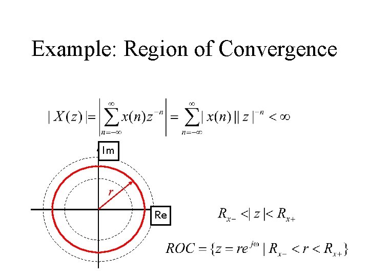
Definition • Give a sequence, the set of values of z for which the z-transform converges, i. e. , |X(z)|< , is called the region of convergence.

Example: Region of Convergence Im r Re

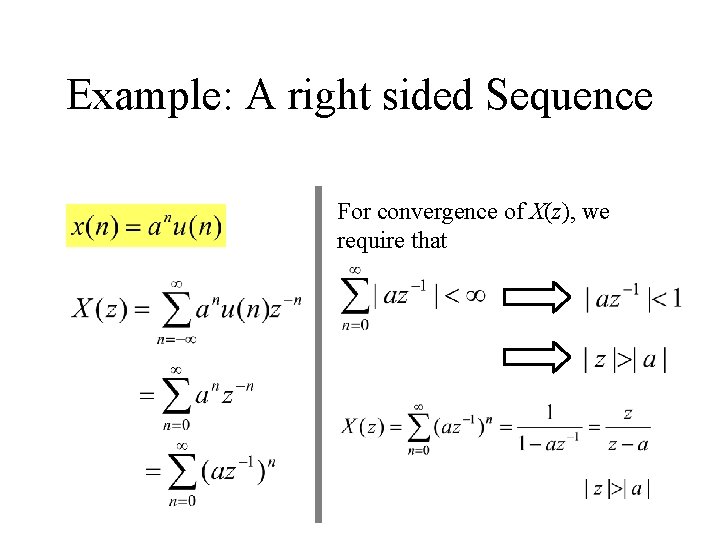
Example: A right sided Sequence For convergence of X(z), we require that

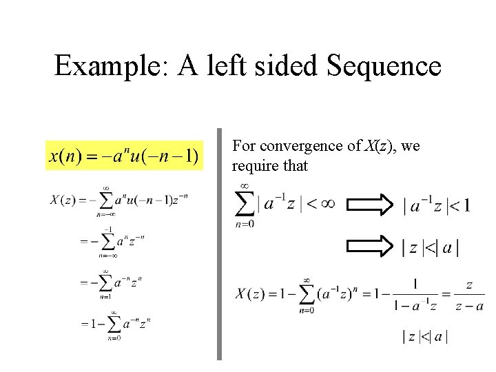
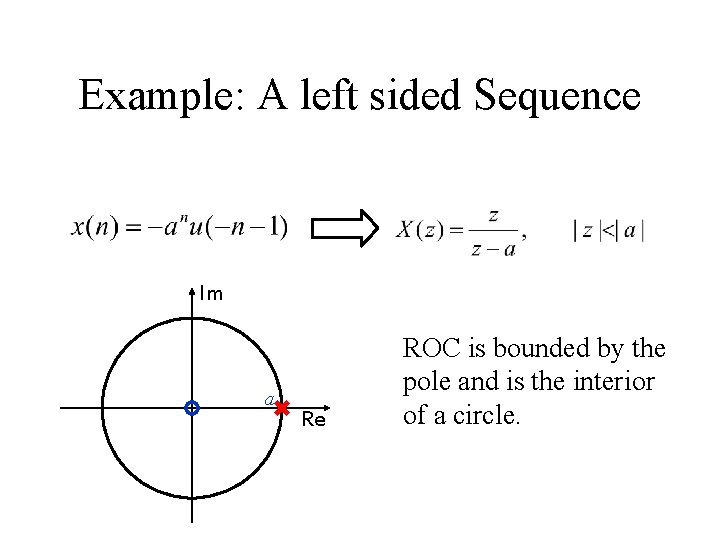
Example: A left sided Sequence For convergence of X(z), we require that

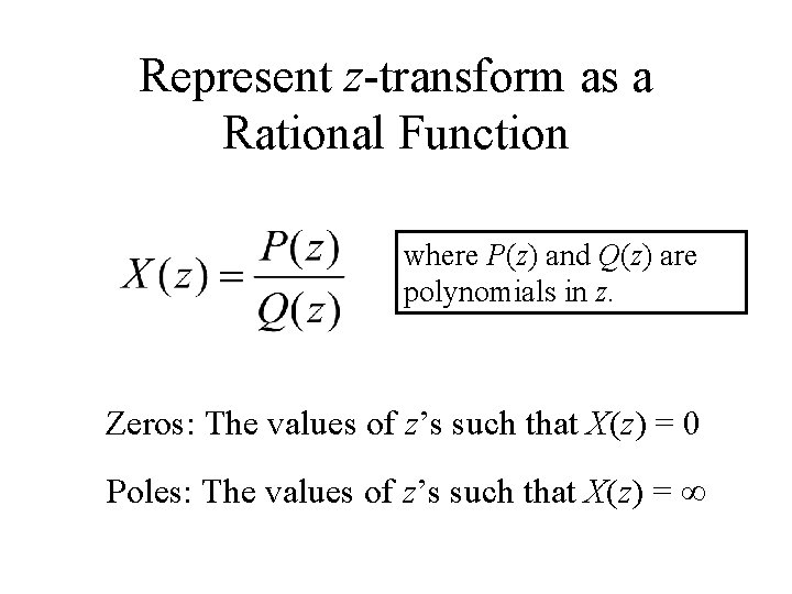
Represent z-transform as a Rational Function where P(z) and Q(z) are polynomials in z. Zeros: The values of z’s such that X(z) = 0 Poles: The values of z’s such that X(z) =

Example: A left sided Sequence Im a Re ROC is bounded by the pole and is the interior of a circle.

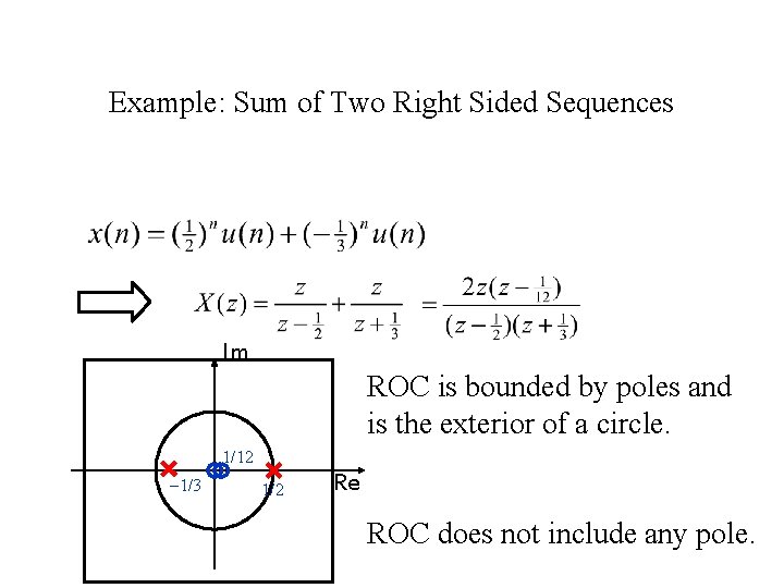
Example: Sum of Two Right Sided Sequences Im ROC is bounded by poles and is the exterior of a circle. 1/12 1/3 1/2 Re ROC does not include any pole.

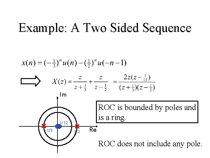
Example: A Two Sided Sequence Im ROC is bounded by poles and is a ring. 1/12 1/3 1/2 Re ROC does not include any pole.

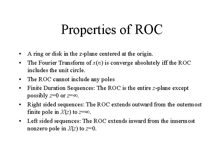
Properties of ROC • A ring or disk in the z-plane centered at the origin. • The Fourier Transform of x(n) is converge absolutely iff the ROC includes the unit circle. • The ROC cannot include any poles • Finite Duration Sequences: The ROC is the entire z-plane except possibly z=0 or z=. • Right sided sequences: The ROC extends outward from the outermost finite pole in X(z) to z=. • Left sided sequences: The ROC extends inward from the innermost nonzero pole in X(z) to z=0.

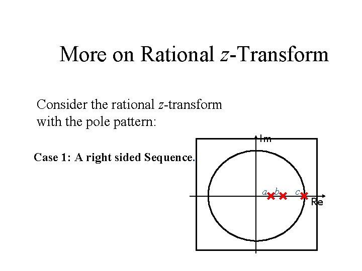
More on Rational z-Transform Consider the rational z-transform with the pole pattern: Im Case 1: A right sided Sequence. a b c Re

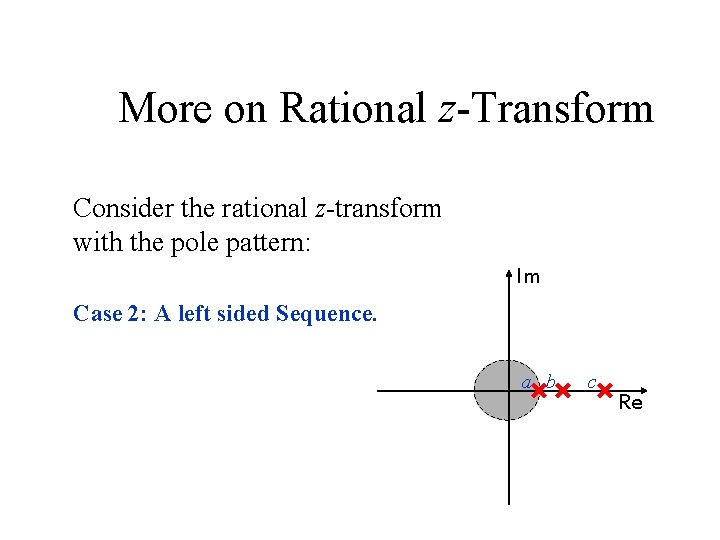
More on Rational z-Transform Consider the rational z-transform with the pole pattern: Im Case 2: A left sided Sequence. a b c Re

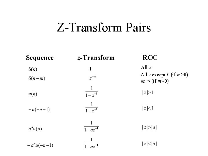
Z-Transform Pairs Sequence z-Transform ROC All z except 0 (if m>0) or (if m<0)

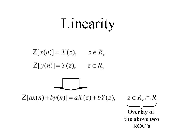
Linearity Overlay of the above two ROC’s

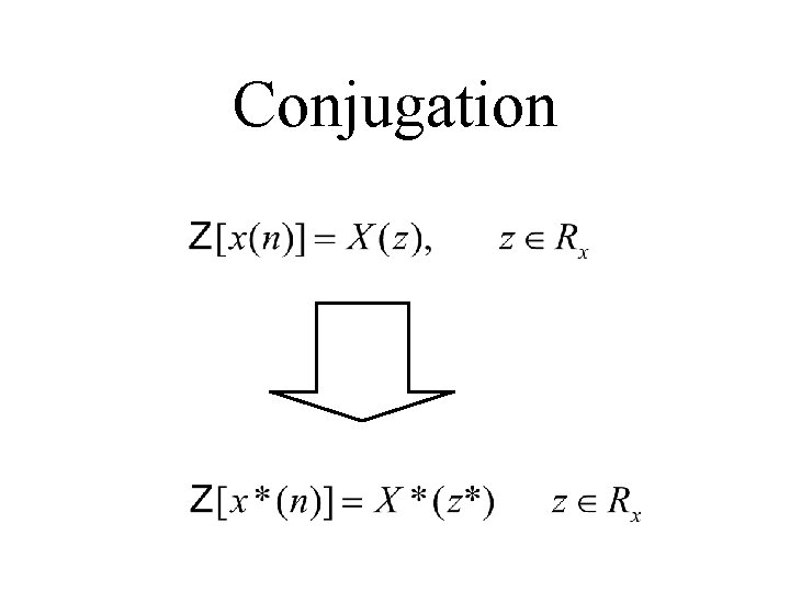
Conjugation

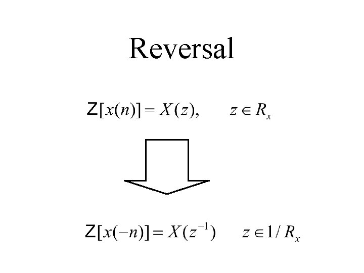
Reversal

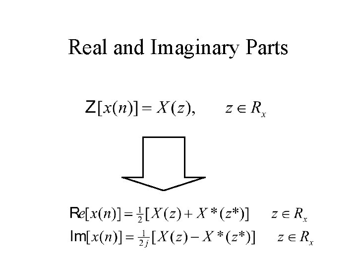
Real and Imaginary Parts

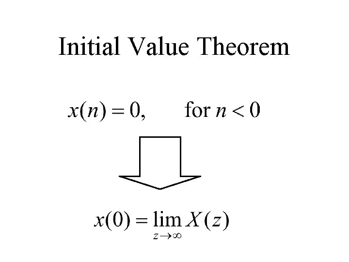
Initial Value Theorem

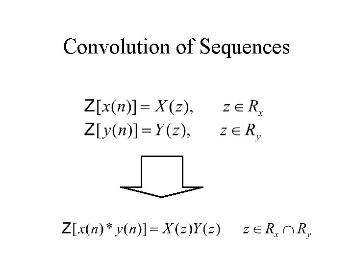
Convolution of Sequences

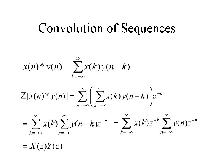
Convolution of Sequences

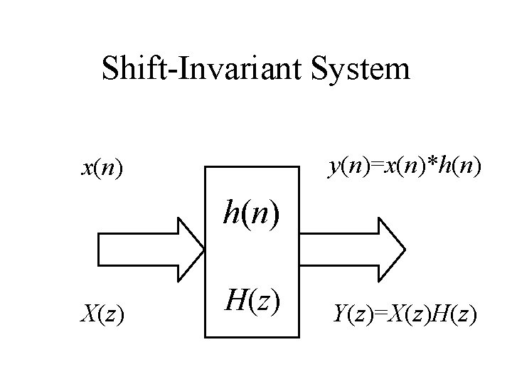
Shift-Invariant System y(n)=x(n)*h(n) x(n) h(n) X(z) H(z) Y(z)=X(z)H(z)

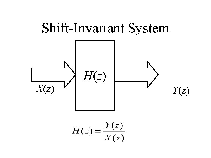
Shift-Invariant System X(z) H(z) Y(z)

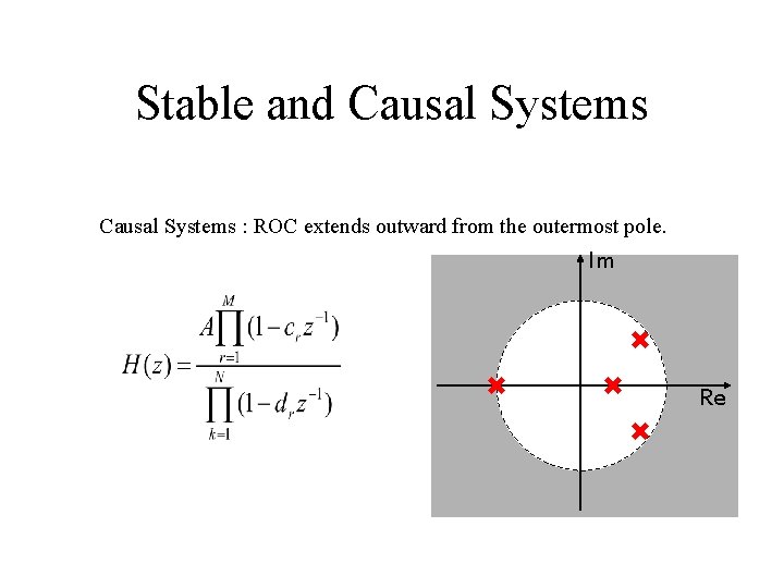
Stable and Causal Systems : ROC extends outward from the outermost pole. Im Re

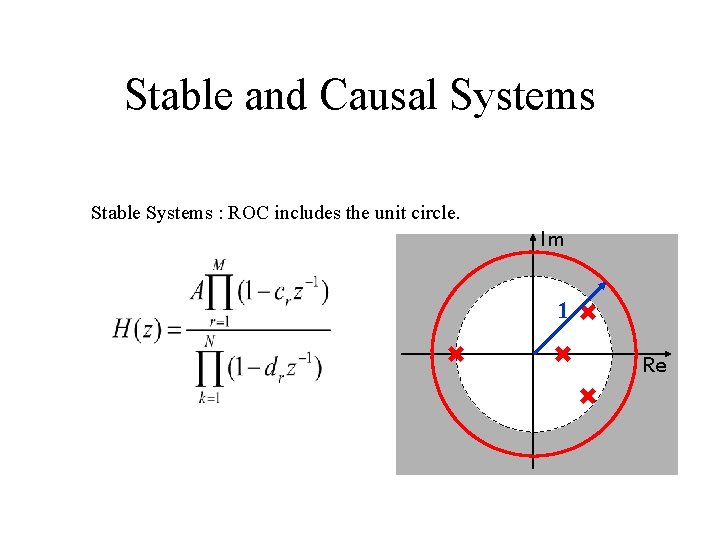
Stable and Causal Systems Stable Systems : ROC includes the unit circle. Im 1 Re

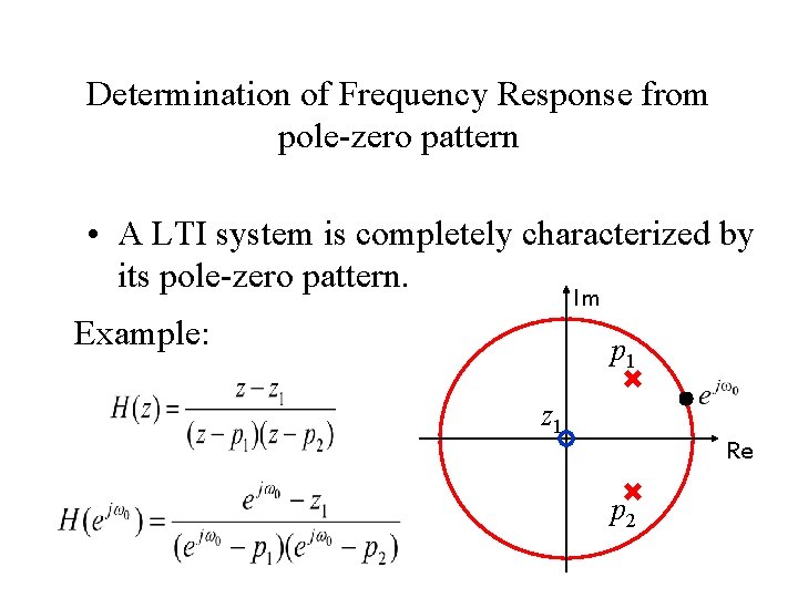
Determination of Frequency Response from pole-zero pattern • A LTI system is completely characterized by its pole-zero pattern. Im Example: p 1 z 1 Re p 2